
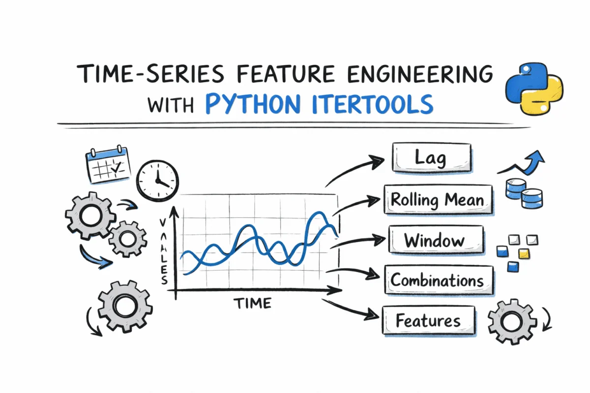
The Distinctive Nature of Time Series Data and Feature Engineering
Time series data, characterized by sequential observations indexed by time, inherently deviates from the assumptions of independence often made for conventional datasets. The chronological order of data points is not merely incidental but central to understanding the underlying processes. Effective feature engineering in this context involves transforming raw time series into a rich set of attributes that encapsulate its temporal patterns, trends, seasonality, and relationships. This includes creating features that reflect:
- Lagged values: Past observations that directly influence future states.
- Rolling statistics: Aggregations over defined time windows to capture local trends, volatility, or typical behavior.
- Temporal interactions: Combinations of different time-based attributes (e.g., hour of day, day of week) to model multi-layered seasonality.
- Rates of change: Derivatives that indicate acceleration or deceleration of a process.
- Cross-series relationships: Correlations or interactions between multiple time series.
- Dynamic baselines: Evolving averages or maximums that provide context for current observations.
Traditional data manipulation libraries, while powerful, can sometimes abstract away the underlying iterative logic needed for such nuanced feature construction. This is where itertools emerges as a highly suitable, low-level alternative, providing a suite of fast, memory-efficient tools for working with iterators.
The itertools Advantage in Data Stream Processing
The itertools module, a standard part of Python’s library, is designed for efficient loop constructions, offering a set of fast, memory-efficient tools for working with iterators. Its functions are built for performance, consuming items one at a time and thus avoiding the creation of large intermediate lists in memory. This "streaming" capability is particularly advantageous when dealing with vast time series datasets where loading the entire history into memory for processing is impractical or inefficient.
While libraries like Pandas offer convenient methods such as .rolling() for common operations, itertools provides the fundamental building blocks, granting data scientists the flexibility to implement highly customized logic for feature generation. This granular control is crucial for tailoring features to specific domain knowledge or complex modeling requirements that might not be directly supported by off-the-shelf functions. The module’s functions are categorized for specific tasks, from infinite iterators to combinatoric generators, each offering a unique approach to sequence manipulation essential for time series analysis.
Crafting Essential Time Series Features: A Methodological Overview
The application of itertools functions to time series feature engineering can be systematically demonstrated across several critical categories. Using a simulated sensor dataset comprising hourly temperature, humidity, and power readings over a week, these methods illustrate how to derive meaningful predictive signals.
1. Generating Lag Features with islice
Lag features represent the value of a variable at a specific point in the past. These are fundamental for capturing autocorrelation and short-term dependencies. For instance, the temperature an hour ago, six hours ago, or 24 hours ago can reveal immediate fluctuations, intra-day patterns, or daily cycles. The itertools.islice() function is ideal for this task. It returns an iterator that yields selected elements from another iterator, effectively "slicing" the sequence without materializing a full copy.
By iterating through a list of desired lag offsets (e.g., 1, 6, 12, 24 hours), islice(sensor_readings, 0, len(sensor_readings) - lag) efficiently extracts the past values. The strategic padding of None or NaN at the beginning of the generated lag series ensures proper alignment with the original time index, a crucial step for subsequent model training where missing values are typically handled. This approach ensures that memory consumption remains minimal, even for very long time series, as only the necessary portion of the data is processed at any given time.
2. Building Rolling Window Features with islice and accumulate
Rolling window statistics provide insights into the behavior of a time series over a defined interval, offering a smoothed perspective that can highlight trends, seasonality, and volatility. Common rolling statistics include mean, standard deviation, minimum, and maximum. Constructing these features efficiently involves both islice for defining the window and itertools.accumulate() for aggregations.
For each point in the time series, a window of a specified size (e.g., 6 hours) is extracted using islice. Within this window, accumulate() can be employed to compute running sums. This function yields successive accumulated results, allowing for the calculation of the sum of the window elements in a single pass. This is particularly efficient for statistics like the mean, where running_sum[-1] / window_size directly provides the result. For other statistics like standard deviation, minimum, and maximum, the window is processed to derive the necessary values. The advantage here lies in avoiding redundant iterations over the window, which can be critical for large datasets or streaming applications.
3. Creating Seasonal Interaction Features with product
Many real-world time series exhibit complex, multi-layered seasonality. For example, energy consumption might vary by hour of the day, day of the week, and whether it’s a holiday. Interaction features combine these temporal dimensions to capture patterns that individual components might miss. itertools.product() is perfectly suited for generating a comprehensive grid of all possible combinations of seasonal factors.
By defining lists for different seasonal components—such as hours_of_day, day_types (weekday/weekend), and operational_shifts (on-peak/off-peak)—itertools.product() can generate every unique combination. This grid can then be used to model baseline expectations or typical behavior for each specific temporal context. For instance, a simulated baseline_temp_c can be calculated for each combination, serving as a powerful feature for anomaly detection (deviation from this baseline). This method ensures that all relevant seasonal interactions are systematically considered, enriching the model’s understanding of periodic variations.
4. Extracting Sliding Window Statistics with tee
In scenarios where multiple statistical measures need to be computed over the same sliding window without redundant iteration or data copying, itertools.tee() becomes invaluable. This function creates multiple independent iterators from a single original iterator.
Consider a need to calculate the mean, range, and rate of change within an 8-hour window for power consumption data. After extracting a window, tee(iter(window)) can generate two or more independent iterators. Each of these new iterators can then be consumed by a different statistical function (e.g., one for sum/mean, another for min/max/range), allowing parallel processing of the window’s elements. This avoids the inefficiency of converting the iterator to a list multiple times or iterating over it repeatedly, thereby optimizing performance, especially for larger windows or when many statistics are required.
5. Combining Multi-Resolution Time Features with chain
Effective time series models often integrate features derived from various temporal resolutions and sources. This might include raw readings, short-term rolling averages, long-term rolling averages, and calendar-derived features (e.g., hour of day, day of week, holiday indicators). Assembling these disparate feature lists into a coherent dataset for modeling can be managed elegantly with itertools.chain().
chain() takes multiple iterables as input and returns a single iterator that yields elements from the first iterable until it is exhausted, then from the second, and so on. This is highly useful for logically grouping and then seamlessly concatenating feature names and their corresponding value lists. For instance, raw humidity, 6-hour rolling humidity, 24-hour rolling humidity, hour of day, and a business hour indicator can all be generated independently. chain() then provides an organized way to combine the names of these features and their respective data arrays into a single, structured input for a Pandas DataFrame, enhancing readability and maintainability of the feature engineering pipeline.
6. Computing Pairwise Temporal Correlations with combinations
In multi-sensor or multivariate time series environments, the dynamic relationships between variables can offer significant predictive power. Synchronous movements or inverse relationships between two sensor readings over time can signal specific operational states or impending events. itertools.combinations() is an effective tool for systematically generating all unique pairs of variables for which to compute such relationships.
Given a list of sensor columns (ee.g., temperature, humidity, power), itertools.combinations(sensor_cols, 2) generates all unique pairs without repetition. For each pair, a rolling window correlation can be calculated. This involves extracting corresponding windows for both series, computing their means and standard deviations, and then calculating the covariance and correlation coefficient. A rolling correlation over a 12-hour window, for example, can reveal how the interrelationship between temperature and humidity or temperature and power evolves over time, providing context-rich features that individual series analyses might overlook.
7. Accumulating Running Baselines with accumulate
The significance of a time series observation is often best understood in relation to its historical context. A deviation from an evolving baseline—such as a running mean or maximum observed so far—can serve as a powerful feature for anomaly detection or trend analysis. itertools.accumulate() is perfectly suited for computing these running statistics efficiently.
By applying accumulate() to the raw readings, one can derive a running sum, which, when divided by a running count (also obtainable via accumulate([1]*len(readings))), yields a running mean. Similarly, accumulate(readings, func=max) efficiently computes the running maximum—the highest value seen up to any point. These running baselines provide a dynamic reference point. A "deviation from baseline" feature (current reading minus running mean) then quantifies how much the current observation departs from its historical average, offering immediate insight into unusual activity without needing to store or re-process the entire history for each new point.
Broader Implications and Future Outlook
The strategic application of Python’s itertools module in time series feature engineering offers a compelling blend of performance, memory efficiency, and programmatic control. By working directly with iterators, data scientists can construct sophisticated temporal features for massive datasets without incurring the memory overhead associated with materializing entire lists. This is particularly relevant in the era of big data and streaming analytics, where processing data in a sequential, memory-conscious manner is paramount.
The ability to precisely define and combine features, as demonstrated across the seven categories, empowers practitioners to move beyond generic solutions and tailor models to the intricate dynamics of their specific time series problems. This granular control often translates into more robust models, improved predictive accuracy, and enhanced interpretability of complex temporal patterns. As time series analysis continues to grow in importance across various industries, from predictive maintenance to financial forecasting, the foundational capabilities offered by itertools will remain an indispensable asset in the data scientist’s toolkit, complementing and extending the functionalities of higher-level libraries. The emphasis on iterable-based processing also positions these techniques well for integration into real-time data pipelines, further solidifying their relevance in an increasingly data-driven world.


Leave a Reply