
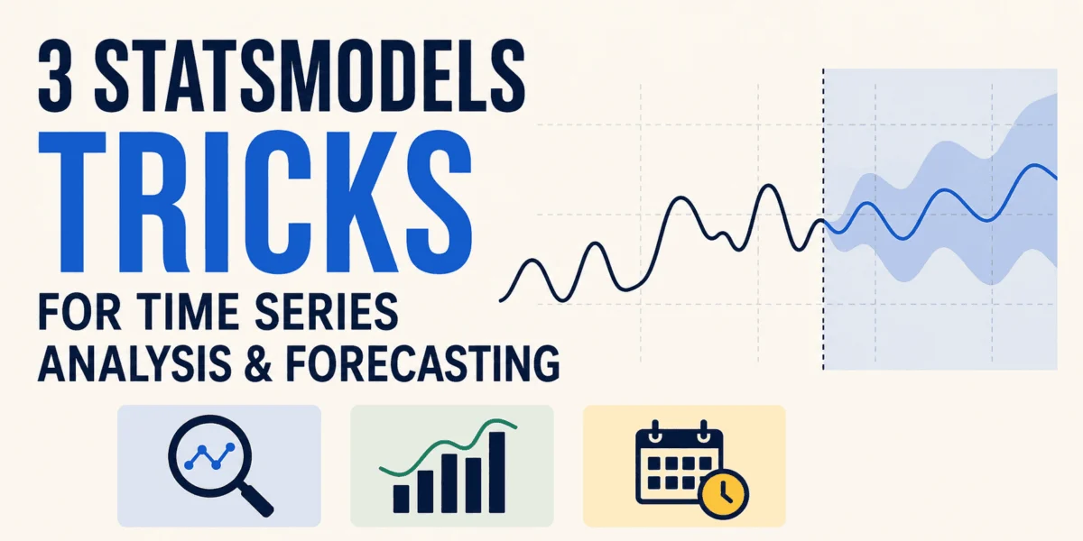
Time series analysis remains one of the most critical yet computationally demanding pillars of modern data science, influencing sectors from macroeconomic forecasting to global supply chain logistics. Within the Python data science ecosystem, Statsmodels has long served as a foundational library, providing robust statistical computations that rival commercial software packages. However, standard developer workflows frequently fail to leverage the full depth of the library’s results objects. When deploying models for production forecasting, engineers routinely rely on rudimentary point-forecast extractions, inadvertently discarding built-in functionalities designed to handle uncertainty estimation, streaming data integration, and complex seasonal decomposition.
A thorough examination of Statsmodels 0.15.0 reveals that fitted models compute far more than simple numeric arrays. By shifting away from hand-rolled scripts and utilizing native methods embedded within the results objects, data practitioners can significantly enhance the reliability, efficiency, and interpretability of their forecasting pipelines.
Background Context and Evolution of Time Series Tooling
The historical trajectory of time series forecasting in Python has evolved from fragmented, custom implementations to standardized, high-performance libraries. Early quantitative analysts frequently relied on manual decomposition techniques, writing bespoke scripts to isolate trend, seasonal, and residual components. While flexible, these home-brewed approaches introduced systemic vulnerabilities, including index misalignment errors, incorrect degrees of freedom, and propagations of sign errors during seasonal adjustments.
The introduction and maturation of libraries like Statsmodels standardized econometric modeling in Python, offering implementations of Autoregressive Integrated Moving Average (ARIMA), Seasonal ARIMA (SARIMAX), and various smoothing techniques. Despite these advancements, empirical observations of production codebases indicate that practitioners often treat fitted models as black boxes. Code is frequently written to extract only the point forecast—the single most basic metric a model can compute—while ignoring the rich statistical metadata accompanying the results object.
To address these inefficiencies, modern data engineering standards emphasize leveraging built-in object methods. Utilizing these native capabilities eliminates redundant computations, reduces codebase complexity, and ensures mathematical consistency across iterative forecasting tasks.
Advanced Interval Estimation: Moving Beyond Point Forecasts
In enterprise environments, presenting a point forecast without a measure of uncertainty is an operational liability. Decision-makers in finance, retail, and energy markets require confidence intervals to formulate risk-mitigation strategies, inventory buffers, and capital allocations.
Standard code implementations frequently request only point estimates through basic indexing or shorthand methods. For example, executing res.forecast(12) yields an array of twelve scalar values. While computationally direct, this approach discards critical variance data that the model has already calculated during the fitting process.
Statsmodels addresses this limitation through the PredictionResults object, accessible via the get_forecast() method. Rather than forcing analysts to manually derive standard errors and confidence bounds, the framework bundles predicted means, standard errors, and upper and lower confidence intervals into a unified data structure.
import statsmodels.api as sm
from statsmodels.tsa.arima.model import ARIMA

# Load and prepare monthly CO2 dataset
co2 = sm.datasets.co2.load_pandas().data["co2"]
co2 = co2.resample("MS").mean().ffill()
train, recent = co2[:-12], co2[-12:]

# Fit the SARIMAX model
res = ARIMA(train, order=(1, 1, 1), seasonal_order=(1, 1, 1, 12)).fit()

# Extract comprehensive prediction frames including confidence intervals
print(res.get_forecast(12).summary_frame().head())
The resulting summary frame provides immediate statistical transparency, outlining exact lower and upper boundaries alongside the primary mean projections. For historical analysis rather than future projections, the get_prediction() method applies an identical architecture to in-sample data periods, allowing auditors to evaluate historical model performance alongside historical uncertainty bounds.
Streamlining Data Updates Without Full Model Retraining
A persistent challenge in operational forecasting pipelines is the arrival of streaming or periodic observations. As new data points accumulate—such as monthly sales figures or quarterly economic indicators—the standard engineering reflex is to concatenate the incoming observations with the historical training set and re-execute the .fit() method from scratch.
While conceptually straightforward, full model retraining is computationally expensive, particularly for complex seasonal ARIMA specifications or high-frequency multivariate datasets. Re-estimating every parameter for every new data batch introduces unnecessary computational overhead and can lead to parameter drift if optimization algorithms converge to slightly different local minima.
Statsmodels mitigates this bottleneck through the .append() method. This functionality updates the existing results object with new observations without necessitating a complete parameter re-estimation, provided the refit=False argument is utilized.
# Append recent observations without re-estimating parameters from scratch
updated = res.append(recent, refit=False)

# Generate updated forecasts incorporating new data
print(updated.get_forecast(6).summary_frame().head())
By default, refit=False preserves the established parameter estimates while seamlessly integrating the new temporal data into the state space matrices. For scenarios where structural breaks occur or sufficient volume accumulates to warrant recalibration, developers can explicitly invoke refit=True. This flexibility allows data architectures to balance computational efficiency with model responsiveness, dynamically adapting to shifting temporal dynamics without incurring unnecessary processing delays.
Automating Seasonal Decomposition with STLForecast
Seasonality remains one of the most pervasive hurdles in time series forecasting. Economic, environmental, and behavioral data frequently exhibit pronounced cyclical patterns that obscure underlying trends. Historically, isolating and correcting for seasonality required a cumbersome, multi-step manual procedure:
- Decomposing the time series into trend, seasonal, and residual components using techniques like Seasonal and Trend decomposition using Loess (STL).
- Manually subtracting or dividing the estimated seasonal component from the original series to generate a deseasonalized dataset.
- Fitting a secondary time series model—such as an ARIMA specification—to the adjusted data, and subsequently manually re-injecting the seasonal component back into the final forecasts.
This manual workflow is notoriously prone to implementation errors, particularly concerning index alignment between seasonal components and forecast horizons. Furthermore, mismatched datetime indices frequently introduce subtle bugs that compromise downstream accuracy.
Statsmodels streamlines this entire procedure through the STLForecast class, encapsulating the decomposition and forecasting pipeline within a single, cohesive object.
from statsmodels.tsa.forecasting.stl import STLForecast

# Instantiate STLForecast with the underlying model class and configuration arguments
stlf = STLForecast(train, ARIMA, model_kwargs="order": (1, 1, 1), "trend": "t")

# Fit and forecast in a single unified workflow
print(stlf.fit().forecast(12).head())
A critical implementation detail often overlooked by practitioners involves the instantiation syntax. Rather than passing a pre-fitted model instance, developers must supply the model class itself—such as ARIMA—alongside its initialization parameters bundled within the model_kwargs dictionary. Passing an already-fitted model represents a frequent source of implementation friction, but adhering to the correct class-reference pattern allows the framework to handle the internal decomposition and forecasting pipeline automatically.
Broader Impact and Implications for Data Infrastructure
The adoption of these native Statsmodels methods carries profound implications for enterprise data architecture and operational efficiency. In large-scale data science operations, inefficient code does not merely consume excess CPU cycles; it introduces maintenance debt, obscures analytical intent, and increases the surface area for production errors.
When development teams rely on hand-rolled scripts to calculate confidence intervals, append streaming data, or execute seasonal decompositions, they assume maintenance responsibility for complex statistical logic that has already been rigorously optimized and tested within established libraries. Conversely, leveraging built-in framework methods aligns codebases with software engineering best practices: reduction of redundant code, adherence to established application programming interfaces (APIs), and maximization of computational efficiency.
Furthermore, as organizations increasingly deploy automated machine learning and continuous forecasting pipelines, the performance gains achieved by avoiding unnecessary model refitting compound significantly. Reducing pipeline latency enables real-time decision-making, ensuring that stakeholders receive timely, accurate, and statistically sound projections.
Future Outlook for Econometric and Statistical Modeling
As the landscape of data science continues to expand into deep learning and transformer-based architectures for time series forecasting, classical statistical frameworks like Statsmodels retain indispensable utility. Their mathematical transparency, interpretability, and rigor make them foundational tools for baseline modeling, causal inference, and regulatory compliance reporting where black-box neural networks are often legally or operationally unviable.
The ongoing maintenance and version evolution of Statsmodels—exemplified by stability improvements in release 0.15.0—underscore the enduring importance of well-architected statistical software. By thoroughly examining results objects, reading comprehensive package documentation, and utilizing native framework methods, data practitioners can elevate the quality of their analyses, ensuring their forecasting pipelines remain mathematically robust, computationally efficient, and resilient against production errors.