
In the fiercely competitive landscape of Silicon Valley, securing a coveted data science or analytics role at tech giants like Meta, Apple, Amazon, Netflix, or Alphabet (collectively known as FAANG) demands far more than rote memorization of statistical definitions. The modern FAANG interview paradigm has shifted dramatically, moving beyond theoretical recall to rigorously assess a candidate’s capacity for critical data analysis, their ability to identify flawed methodologies, and their judgment in preventing erroneous insights from impacting production systems. At the heart of this evaluation lie statistical traps – carefully crafted scenarios designed to mimic real-world analytical dilemmas that can derail even the most mathematically adept professionals. These pitfalls serve as a reliable litmus test for discerning true data acumen from superficial understanding.
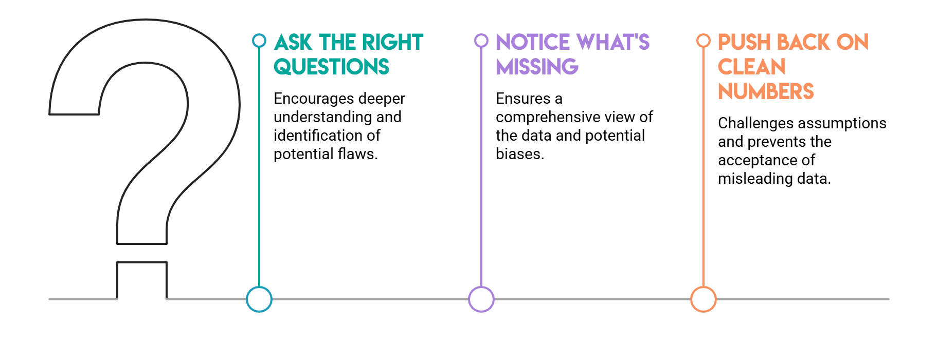
The challenges presented in these interviews are not academic curiosities; they are direct reflections of the daily decisions faced by data analysts and scientists within these organizations. Picture a dashboard metric that appears benign but masks a critical underlying issue, or an A/B test result that seems actionable yet harbors a structural flaw. Interviewers, already privy to the correct answers, meticulously observe the candidate’s thought process. They scrutinize the questions asked, the identification of missing information, and the willingness to challenge seemingly favorable numbers. It is a common observation that candidates, despite robust academic backgrounds, frequently stumble over these nuanced statistical hurdles. This article will delve into five of the most prevalent and insidious statistical traps encountered in FAANG interviews, offering a comprehensive look at their nature, implications, and how seasoned professionals navigate them.
The Deceptive Aggregation: Understanding Simpson’s Paradox
One of the most common statistical traps, Simpson’s Paradox, is specifically designed to identify candidates who uncritically accept aggregated data. This phenomenon occurs when a trend observed within different subgroups of data disappears or reverses when these groups are combined. The quintessential illustration of this paradox stems from UC Berkeley’s 1973 graduate admissions data, which initially suggested a bias against women. The overall admission rates appeared to favor men; however, upon disaggregating the data by individual departments, women were found to have equal or even superior admission rates. The aggregate figure was profoundly misleading, primarily because women disproportionately applied to more competitive departments with lower overall admission rates.
The core of Simpson’s Paradox lies in the interplay of differing group sizes and varying base rates across those groups. A deep understanding of this underlying mechanism is what distinguishes a superficial answer from a truly insightful one. In an interview setting, a typical scenario might be posed: "We conducted an A/B test for a new feature. Overall, Variant B showed a higher conversion rate. Yet, when we segmented the results by device type, Variant A performed better on both mobile and desktop. How do you explain this discrepancy?" A strong candidate would immediately recognize the hallmarks of Simpson’s Paradox. They would articulate its cause—namely, that the distribution of user traffic across device types likely differed significantly between Variant A and Variant B, with Variant B potentially receiving a larger proportion of traffic from the higher-converting mobile segment. Crucially, they would request a detailed breakdown of conversion rates and visitor counts by variant and device type, rather than blindly trusting the aggregate figure.
The implications of overlooking Simpson’s Paradox in real-world A/B testing at FAANG scale are substantial. Launching a feature based solely on an aggregate positive result, only to discover it underperforms in key user segments, can lead to wasted development resources, negative user experiences, and a misallocation of marketing spend. Interviewers use this trap to gauge a candidate’s instinctive inclination to probe subgroup distributions and to challenge high-level metrics. Failing to question the aggregate number invariably results in lost points, signaling a potential blind spot in critical data interpretation.
Consider this Python demonstration of how aggregate rates can be misleading:
import pandas as pd

# A wins on both devices individually, but B wins in aggregate
# because B gets most traffic from higher-converting mobile.
data = pd.DataFrame(
    'device':   ['mobile', 'mobile', 'desktop', 'desktop'],
    'variant':  ['A', 'B', 'A', 'B'],
    'converts': [40, 765, 90, 10],
    'visitors': [100, 900, 900, 100],
)
data['rate'] = data['converts'] / data['visitors']

print('Per device:')
print(data[['device', 'variant', 'rate']].to_string(index=False))
print('nAggregate (misleading):')
agg = data.groupby('variant')[['converts', 'visitors']].sum()
agg['rate'] = agg['converts'] / agg['visitors']
print(agg['rate'])
Output:
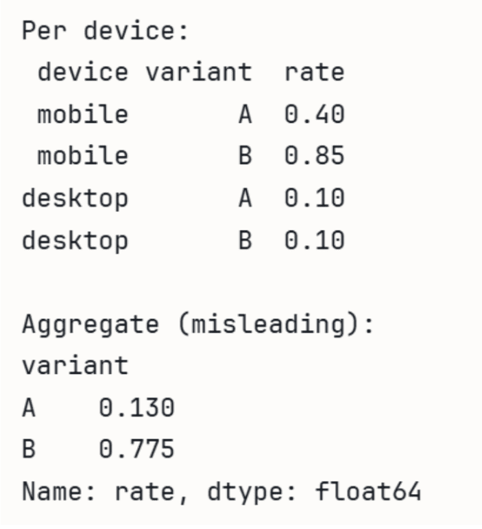
Per device:
 device variant  rate
 mobile       A  0.40
 mobile       B  0.85
desktop       A  0.10
desktop       B  0.10

Aggregate (misleading):
variant
A    0.13
B    0.85
Name: rate, dtype: float64
In this example, Variant A has a 40% conversion rate on mobile and 10% on desktop, while Variant B has 85% on mobile and 10% on desktop. Individually, A performs worse than B on mobile (0.40 vs 0.85) but ties on desktop (0.10 vs 0.10). However, the aggregate shows B winning significantly because it received 900 visitors on mobile (where its rate is high) compared to A’s 100 mobile visitors. This illustrates the critical need to examine underlying distributions.
The Source of Truth: Identifying Selection Bias
This particular test allows interviewers to assess a candidate’s foundational understanding of data provenance – the origin and collection methodology of the data – before any analysis commences. Selection bias is a pervasive and often insidious issue, arising when the data available for analysis is not truly representative of the broader population or phenomenon one intends to study. Its danger lies in its origin within the data collection process itself, making it deceptively easy to overlook during the analytical phase.
Consider various interview framings that expose this trap: "Our user survey shows extremely high satisfaction rates with a recently launched feature. Should we allocate more resources to similar features?" or "We observed that customers who opt-in to our email newsletter have significantly higher lifetime value. Should we aggressively push newsletter sign-ups to all users?" A candidate who immediately recommends action based on these correlations without scrutinizing the data source is likely to fall into the trap.
A closely related and equally important variant is survivorship bias. This occurs when an analysis is conducted only on data that has "survived" a particular filtering process, leading to a skewed perspective. For instance, if a company only analyzes the characteristics of its most successful products to understand what made them thrive, it risks ignoring the identical characteristics present in products that ultimately failed. This leads to attributing success to factors that are merely common, not causal, and can result in misguided strategic decisions. For example, analyzing only the features of top-performing apps in an app store might lead to conclusions that ignore the vast majority of apps with similar features that did not succeed.
Simulating non-response bias can illustrate how results are skewed:
import numpy as np
import pandas as pd

np.random.seed(42)
# Simulate users where satisfied users are more likely to respond
satisfaction = np.random.choice([0, 1], size=1000, p=[0.5, 0.5])
# Response probability: 80% for satisfied, 20% for unsatisfied
response_prob = np.where(satisfaction == 1, 0.8, 0.2)
responded = np.random.rand(1000) < response_prob

print(f"True satisfaction rate: satisfaction.mean():.2%")
print(f"Survey satisfaction rate: satisfaction[responded].mean():.2%")
Output:
True satisfaction rate: 50.00%
Survey satisfaction rate: 80.00%
Here, the true satisfaction rate is 50%, but due to satisfied users being far more likely to respond, the survey reports a misleading 80% satisfaction.
The consequences of selection bias at a FAANG company can be severe. Misinterpreting user sentiment due to a biased survey sample could lead to building features that only a subset of highly engaged users desires, alienating the broader user base. Similarly, drawing conclusions about overall market trends from data skewed by a specific geographic region or demographic can result in flawed product roadmaps and ineffective marketing campaigns. Interviewers leverage selection bias questions to gauge a candidate’s ability to differentiate between "what the data shows" and "what is true about the user population." A strong candidate would probe the sampling methodology, consider potential confounding factors in survey participation, or question the generalizability of observed correlations, demonstrating a holistic understanding of data validity.
The Peril of Post-Hoc Significance: Preventing p-Hacking
P-hacking, also known as data dredging or fishing for significance, represents a critical ethical and methodological pitfall in statistical analysis. It occurs when researchers or analysts conduct numerous statistical tests and selectively report only those results that achieve a predetermined level of statistical significance (typically a p-value less than 0.05). The fundamental issue stems from a misunderstanding or misuse of p-values, which are designed for individual hypothesis tests, not for a battery of exploratory analyses.
By definition, a p-value of 0.05 implies a 5% chance of observing a result as extreme as, or more extreme than, the one obtained, assuming the null hypothesis is true. This means that if 20 independent tests are conducted under the null hypothesis (i.e., there is no real effect), one would statistically expect at least one false positive result purely by chance. P-hacking dramatically inflates the false discovery rate by systematically searching for significant results, thereby eroding the reliability and credibility of scientific findings and business insights. This practice contributed significantly to the "reproducibility crisis" in various scientific fields, where many published findings could not be replicated by independent researchers.
An interviewer might present a scenario such as: "Last quarter, our product team conducted fifteen different feature experiments. Three of these experiments yielded statistically significant results at a p-value of 0.05. Do all three features necessarily warrant shipping to production?" A weak candidate might confidently affirm that all three should be shipped, indicating a lack of understanding of p-hacking and multiple comparisons.
A strong candidate, however, would immediately question the methodology. They would inquire about the pre-registration of hypotheses – whether the specific hypotheses for each of the fifteen experiments were defined before data collection began. They would also ask if the significance threshold was established in advance for each test, and crucially, whether any statistical correction for multiple comparisons was applied. The follow-up discussion often revolves around best practices for designing experiments to circumvent p-hacking. The most direct and robust solution is the pre-registration of hypotheses and analysis plans, which eliminates the opportunity to retroactively decide which tests were "real" or to cherry-pick favorable outcomes. This commitment to transparency and pre-specification is a hallmark of rigorous data science.
Observing how false positives accumulate by chance:
import numpy as np
from scipy import stats
np.random.seed(0)

# 20 A/B tests where the null hypothesis is TRUE (no real effect)
n_tests, alpha = 20, 0.05
false_positives = 0

for _ in range_n_tests:
    a = np.random.normal(0, 1, 1000)
    b = np.random.normal(0, 1, 1000)  # identical distribution!
    if stats.ttest_ind(a, b).pvalue < alpha:
        false_positives += 1

print(f'Tests run:                 n_tests')
print(f'False positives (p<0.05): false_positives')
print(f'Expected by chance alone: n_tests * alpha:.0f')
Output:
Tests run:                 20
False positives (p<0.05): 1
Expected by chance alone: 1
This simulation demonstrates that even when there is absolutely no real difference between groups (i.e., the null hypothesis is true), a p-value less than 0.05 will occur by chance approximately 5% of the time. If a product team runs 15 experiments and selectively highlights only the "significant" ones, there’s a high probability that these results are merely statistical noise. It is equally vital to distinguish between exploratory data analysis (which generates hypotheses) and confirmatory experiments (which test them). Any actionable insights derived from exploratory analysis should always be validated through a new, pre-registered confirmatory experiment before being implemented at scale.
The Statistical Inflation: Managing Multiple Testing
Closely related to p-hacking, yet a distinct formal statistical challenge, is the multiple testing problem. This issue arises intrinsically when conducting numerous hypothesis tests simultaneously, as the probability of incurring at least one false positive (a Type I error) escalates rapidly with each additional test. Even if the underlying treatment or intervention has no genuine effect, one should anticipate approximately five false positives if 100 different metrics are monitored in a single A/B test and any metric with a p-value below 0.05 is declared significant. The "family-wise error rate" – the probability of making at least one Type I error in a set of inferences – grows much faster than the individual test alpha level.
Fortunately, well-established statistical corrections exist to mitigate the multiple testing problem. The Bonferroni correction is a highly conservative approach, which involves dividing the original alpha level by the number of tests performed. For example, if 50 metrics are being tested, the per-test significance threshold drops from 0.05 to 0.001 (0.05/50). While effective at controlling the family-wise error rate, Bonferroni correction significantly reduces statistical power, making it harder to detect true effects, especially subtle ones. A less conservative, and often more appropriate, method is the Benjamini-Hochberg procedure, which controls the False Discovery Rate (FDR) rather than the family-wise error rate. FDR is the expected proportion of false positives among all rejected null hypotheses. Benjamini-Hochberg is particularly useful when one is willing to accept a certain proportion of false discoveries in exchange for greater statistical power and a higher chance of identifying real effects.
In FAANG interviews, this problem often surfaces when discussing the rigorous tracking and interpretation of experiment metrics. A common question might be: "Our experimentation platform tracks 50 different metrics for every A/B test we run. How do you determine which of these metrics truly ‘matter’ when evaluating an experiment?" A robust response would articulate the importance of pre-specifying primary metrics – the key performance indicators (KPIs) that directly address the core hypothesis – before the experiment is launched. Secondary metrics should then be treated as exploratory, with a clear acknowledgment of the multiple testing problem and the need for appropriate corrections or subsequent confirmatory tests if interesting signals emerge.
Interviewers use this question to gauge a candidate’s awareness that simply accumulating more tests does not necessarily equate to more reliable information; rather, it often introduces more statistical noise. A candidate who understands the nuances of multiple comparisons demonstrates a crucial ability to prioritize, strategize, and interpret experimental results responsibly in a data-rich environment.
The Illusion of Influence: Addressing Confounding Variables
This trap is designed to catch candidates who hastily equate correlation with causation without diligently investigating alternative explanations for observed relationships. A confounding variable is a factor that exerts influence on both the independent variable (the cause being studied) and the dependent variable (the effect being measured), thereby creating a spurious or illusory association between the two.
The classic illustrative example involves the positive correlation between ice cream sales and drowning rates. A naive interpretation might suggest that ice cream consumption leads to drowning. However, the confounder in this relationship is summer heat; both ice cream sales and swimming activities (and thus, tragically, drowning incidents) increase during warmer months. Acting on the direct correlation without accounting for this confounder would lead to absurd and ineffective policy recommendations.
Confounding is particularly dangerous when analyzing observational data, as opposed to data from randomized controlled experiments. In observational studies, researchers merely observe existing patterns without manipulating variables. Unlike randomized experiments, which ideally distribute potential confounders evenly across treatment and control groups, observational data does not inherently control for such factors. Consequently, any differences observed between groups might not be caused by the variable under investigation but by unmeasured or uncontrolled confounders.

A typical interview framing might be: "We’ve noticed a strong correlation: users who engage with our mobile app more frequently tend to generate significantly higher revenue. Based on this, should we implement a strategy to push more notifications to increase app opens, expecting a boost in revenue?" A weak candidate might enthusiastically endorse this strategy. A strong candidate, however, would immediately question the causal direction. They would inquire about the characteristics of users who frequently open the app to begin with. It is highly probable that these are already the most engaged, highest-value users – individuals whose inherent interest and loyalty drive both their frequent app usage and their higher spending. In this scenario, engagement itself is the underlying confounder, driving both app opens and revenue. The app opens are not causing the revenue; they are a symptom of the same underlying user quality.
Simulating a confounded relationship provides clarity:
import numpy as np
import pandas as pd
np.random.seed(42)
n = 1000
# Confounder: user quality (0 = low, 1 = high)
user_quality = np.random.binomial(1, 0.5, n)
# App opens driven by user quality, not independent
app_opens = user_quality * 5 + np.random.normal(0, 1, n)
# Revenue also driven by user quality, not app opens
revenue = user_quality * 100 + np.random.normal(0, 10, n)
df = pd.DataFrame(
    'user_quality': user_quality,
    'app_opens': app_opens,
    'revenue': revenue
)
# Naive correlation looks strong – misleading
naive_corr = df['app_opens'].corr(df['revenue'])
# Within-group correlation (controlling for confounder) is near zero
corr_low  = df[df['user_quality']==0]['app_opens'].corr(df[df['user_quality']==0]['revenue'])
corr_high = df[df['user_quality']==1]['app_opens'].corr(df[df['user_quality']==1]['revenue'])
print(f"Naive correlation (app opens vs revenue): naive_corr:.2f")
print(f"Correlation controlling for user quality:")
print(f"  Low-quality users:  corr_low:.2f")
print(f"  High-quality users: corr_high:.2f")
Output:
Naive correlation (app opens vs revenue): 0.91

Correlation controlling for user quality:

  Low-quality users:  0.03
  High-quality users: -0.07
The initial correlation between app opens and revenue appears strikingly strong at 0.91. However, once the analysis controls for the confounding variable of ‘user quality’ (by examining correlations within low-quality and high-quality user groups separately), the relationship between app opens and revenue virtually disappears. This stark contrast underscores the critical importance of identifying and accounting for confounders. Interviewers who observe a candidate performing this kind of stratified analysis, rather than accepting the aggregate correlation at face value, gain confidence that they are speaking with a professional who will provide robust, actionable recommendations and avoid shipping flawed product decisions. They are looking for candidates who understand that randomized experimentation is the gold standard for establishing causality, and in situations where randomization isn’t feasible, techniques like propensity score matching or instrumental variables should be considered.
Broader Implications and Industry Best Practices
These five statistical traps – Simpson’s Paradox, Selection Bias, P-Hacking, Multiple Testing, and Confounding Variables – share a fundamental commonality: they demand a disciplined approach to data analysis that prioritizes critical inquiry and skepticism over immediate acceptance of numerical outputs. In the fast-paced, data-intensive environments of FAANG companies, the ability to "slow down and question the data" is not merely an academic exercise; it is an essential safeguard against costly errors.
The stakes are incredibly high. A misinterpretation of A/B test results due to Simpson’s Paradox could lead to the rollout of features that actively degrade user experience for significant segments. Unaddressed selection bias in user feedback could result in product development catering to a vocal minority, alienating the broader user base. The unchecked pursuit of "significant" results through p-hacking or ignoring multiple testing corrections can lead to the allocation of millions of dollars in engineering resources to features with no real impact, eroding developer trust and wasting valuable time. And mistaking correlation for causation due to confounding variables can result in product strategies based on false premises, failing to move key business metrics.

Leading tech companies invest heavily in robust experimentation platforms, sophisticated data governance frameworks, and continuous training for their data professionals precisely because these traps are common failure modes in real-world data work. They foster a culture of data literacy and critical thinking, encouraging analysts to be "data skeptics" who rigorously validate assumptions and results.
For aspiring data professionals eyeing a career at FAANG, developing a reflex to ask probing questions is paramount. This includes inquiring about data collection methodologies, potential biases in sampling, the pre-registration of hypotheses for experiments, the number of metrics being tested, and the potential presence of confounding variables. These habits extend beyond interview success; they are the bedrock of responsible, impactful data science. The candidate who can instinctively recognize Simpson’s Paradox in a product metric, flag a selection bias in a survey, question the validity of an experiment result against multiple comparisons, or distinguish correlation from causation will be the professional who consistently makes fewer bad decisions and, consequently, drives more meaningful innovation. In an era where data underpins every strategic move, mastering these statistical nuances is not just an advantage—it is a necessity.


Leave a Reply