


The realm of modern data analysis is characterized by an ever-increasing volume and complexity of data, demanding robust and efficient tools for extraction, transformation, and insight generation. At the forefront of this analytical revolution stands Pandas, a cornerstone library within the Python ecosystem, widely celebrated for its intuitive yet powerful capabilities in handling structured data. Among its diverse functionalities, the GroupBy operation emerges as a particularly indispensable feature, fundamentally reshaping how data professionals approach complex aggregations and multi-dimensional analysis. This mechanism, deeply rooted in the "split-apply-combine" paradigm, empowers users to segment datasets based on specific criteria, perform calculations on these isolated segments, and then reassemble the results into a coherent, insightful summary.
The Strategic Imperative of GroupBy in Modern Data Science

In an era where data-driven decision-making is paramount, the ability to quickly and accurately summarize information is critical. Businesses, researchers, and analysts across sectors—from retail and finance to healthcare and scientific research—grapple daily with large datasets containing granular transactional details, customer demographics, sensor readings, or experimental outcomes. Questions such as "What is the total revenue generated by each sales region?", "Which product categories are performing best in specific markets?", or "How does customer behavior vary across different age groups?" are common. Manually filtering and calculating these metrics for each category would be an arduous, error-prone, and computationally inefficient task. This is precisely where Pandas GroupBy provides a transformative solution, offering a streamlined, declarative approach to these challenges. Its efficiency and flexibility have cemented its status as an industry standard for aggregating and exploring structured data, allowing data professionals to transition from manual, iterative processes to automated, scalable analytical workflows.
Foundational GroupBy Operations: The Split-Apply-Combine Paradigm
At its core, the GroupBy operation adheres to a three-step process:
- Splitting: The data is divided into groups based on one or more keys. For instance, in a sales dataset, this might involve separating all transactions by
regionorproduct category. - Applying: A function is applied independently to each group. This could be an aggregation function (like sum, mean, count), a transformation function (like standardization), or a filtration function.
- Combining: The results of these individual operations are merged back into a single data structure, typically a Pandas DataFrame or Series.
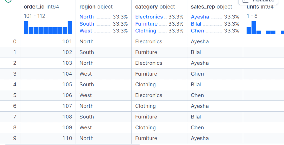
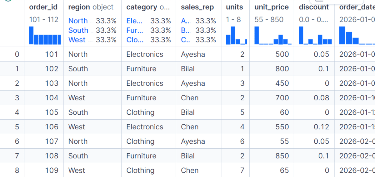
To illustrate these foundational principles, consider a typical retail sales dataset. This dataset might include order_id, region, category, sales_rep, units sold, unit_price, discount, and order_date. From this raw data, derived metrics like gross_sales (units unit_price) and net_sales (gross_sales (1 – discount)) are often calculated to provide a comprehensive view of transactional value.
A fundamental application of GroupBy involves calculating total net_sales for each region. The syntax is remarkably concise: df.groupby("region")["net_sales"].sum(). This operation immediately yields a Series where each region is an index, and its corresponding value represents the aggregated net sales. For reporting or subsequent data manipulation, it is often more convenient to have the grouped column as a regular column rather than an index. The as_index=False parameter, as in df.groupby("region", as_index=False)["net_sales"].sum(), addresses this by returning a DataFrame, making the output directly amenable for further processing or visualization. Industry analysts frequently cite this feature as crucial for maintaining clean, interoperable data structures within complex analytical pipelines.
Advanced Aggregation and Customization: Beyond Simple Sums

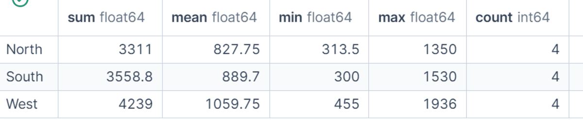
The utility of GroupBy extends far beyond simple summations. Data analysts often require a more comprehensive statistical overview of their groups. Pandas facilitates this through the agg() method, which allows for the application of multiple aggregation functions to the same column or different columns simultaneously. For example, to obtain a statistical summary of net_sales for each region, one might calculate the sum, mean, minimum, maximum, and count of sales using df.groupby("region")["net_sales"].agg(["sum", "mean", "min", "max", "count"]). This provides immediate insights into not just total revenue, but also average transaction value, the range of sales figures, and the volume of orders within each region, offering a quick diagnostic of regional performance.
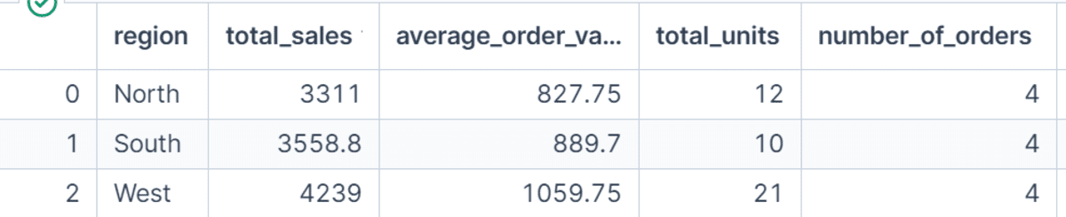
For enhanced clarity and report readability, especially in complex analyses involving numerous metrics, Pandas offers "named aggregations." Instead of generic column names like ‘sum’ or ‘mean’ in the output, users can define descriptive names such as total_sales, average_order_value, total_units, or number_of_orders. This is achieved by passing keyword arguments to agg(), where each keyword specifies the new column name, and its value is a tuple containing the source column and the aggregation function (e.g., total_sales=("net_sales", "sum")). This feature is invaluable when preparing data for dashboards, executive reports, or machine learning feature engineering, ensuring that the derived metrics are self-explanatory and immediately actionable.
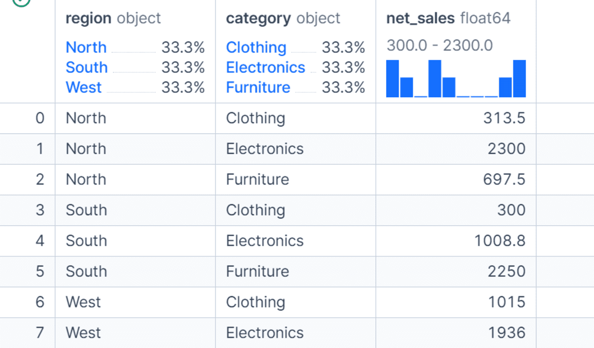
Furthermore, real-world data analysis frequently necessitates segmentation across multiple dimensions. GroupBy seamlessly supports grouping by more than one column, allowing for intricate multi-dimensional insights. For instance, df.groupby(["region", "category"], as_index=False)["net_sales"].sum() would calculate total net sales for each product category within each region. This granular view is essential for understanding performance variations across different segments, such as identifying top-selling categories in specific geographical markets or analyzing sales representative performance within different product lines. Such multi-level insights are critical for strategic planning, resource allocation, and targeted marketing campaigns.
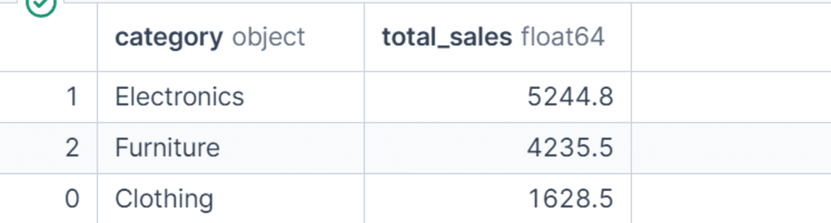
Once data is grouped and aggregated, sorting the results is a common subsequent step to highlight key findings. After calculating total sales by product category, for example, sorting the results in descending order of total_sales (using .sort_values("total_sales", ascending=False)) quickly reveals the highest-revenue-generating categories. This simple yet powerful step transforms raw aggregated data into actionable intelligence, making it easier to pinpoint top performers or areas requiring attention.
Nuances in Group Counting: count() vs. size()
A subtle but important distinction exists between count() and size() within GroupBy operations. While both relate to counting elements within groups, their behavior differs regarding missing values. The size() method counts the total number of rows (observations) in each group, including those with NaN (Not a Number) or None values. In contrast, the count() method, when applied to a specific column, only tallies the non-missing values within that column for each group.
This distinction becomes critical in data quality assessments and ensuring accurate statistical representation. If, for instance, a dataset contains missing sales_rep information for certain orders, df.groupby("region").size() would still report the full number of orders per region, whereas df.groupby("region")["sales_rep"].count() would return a lower count for regions affected by missing sales_rep data. Understanding this difference is vital for data integrity, as misinterpreting these counts could lead to flawed conclusions regarding group sizes or data completeness.
Extending GroupBy: transform(), filter(), and apply()
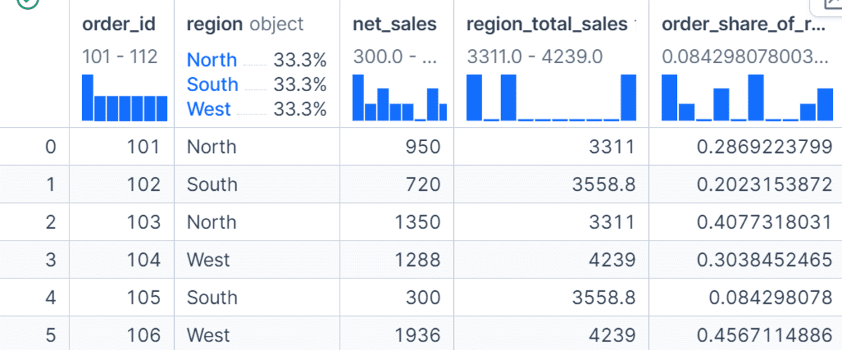
Beyond direct aggregation, Pandas GroupBy offers advanced methods for more complex group-wise operations. The transform() method is particularly powerful for enriching the original DataFrame with group-level information. Unlike agg(), which reduces each group to a single summary row, transform() returns a Series or DataFrame that has the same index as the original DataFrame, with values aligned to the original rows. This means a group-level statistic, such as the total sales for a region, can be broadcast back to every individual order within that region. For example, calculating df["region_total_sales"] = df.groupby("region")["net_sales"].transform("sum") allows for the subsequent computation of each order’s order_share_of_region by dividing net_sales by region_total_sales. This capability is immensely valuable in feature engineering for machine learning models, where individual data points are often contextualized by their group’s characteristics.
The filter() method enables the selection or exclusion of entire groups based on specific conditions. Instead of returning aggregated summaries, filter() returns the original rows belonging only to the groups that satisfy the defined criteria. For instance, to analyze only regions exceeding a certain sales threshold, one could use df.groupby("region").filter(lambda group: group["net_sales"].sum() > 3000). This technique is widely applied in scenarios like identifying high-performing customer segments, flagging underperforming branches, or filtering out groups that do not meet minimum data quality standards, allowing analysts to focus on relevant subsets of their data.
For operations that do not fit neatly into built-in aggregation, transformation, or filtering functions, the apply() method provides maximum flexibility. It allows users to execute custom logic on each group, returning either a Series or DataFrame based on the custom function’s output. An example includes finding the top order by net sales within each region using df.groupby("region", group_keys=False).apply(lambda group: group.nlargest(1, "net_sales")). While apply() is incredibly versatile, data scientists frequently advise caution regarding its performance characteristics, as it can be slower than vectorized built-in methods, especially on very large datasets. It is best reserved for operations where no equivalent optimized Pandas function exists.
Temporal Analysis with GroupBy: Mastering Date-Based Grouping
Time-series data forms a significant portion of real-world datasets, and GroupBy is exceptionally adept at facilitating temporal analysis. Extracting components like the month or year from a datetime column and then grouping by these new features is a common practice. For instance, df["month"] = df["order_date"].dt.to_period("M").astype(str) creates a new column representing the month, enabling df.groupby("month").agg(total_sales=("net_sales", "sum"), total_orders=("order_id", "count")) for monthly sales and order summaries. This method is fundamental for uncovering seasonal trends, identifying periods of peak activity, or analyzing growth over time.
For a more streamlined and robust approach to time-series grouping, Pandas offers pd.Grouper. This powerful object allows grouping by a datetime index or column at specified frequencies (e.g., ‘D’ for day, ‘W’ for week, ‘M’ for month, ‘Q’ for quarter, ‘Y’ for year) without the need to manually extract date components. Using df.groupby(pd.Grouper(key="order_date", freq="M")) provides a clean and efficient way to summarize data by month, directly producing a time-indexed result. This capability is indispensable for financial reporting, epidemiological studies, climate data analysis, and any domain where understanding temporal patterns is crucial. Data professionals commend pd.Grouper for its elegance and efficiency in handling diverse time-based aggregations, significantly simplifying what would otherwise be complex date manipulation tasks.
Reshaping Data for Insight: Pivot-Style Summaries
Beyond simple tabular outputs, GroupBy can be combined with unstack() to generate pivot-style summary tables, which are invaluable for comparative analysis and reporting. By grouping data by two columns (e.g., region and category), aggregating a value (e.g., net_sales), and then using unstack(fill_value=0) to transform one of the grouping levels into columns, a cross-tabulated view is created. This region_category_table provides an immediate, clear comparison of sales performance for each product category across different regions. Such compact and readable tables are highly favored in business intelligence for quickly identifying performance disparities, understanding market distribution, and supporting strategic decisions.
Broader Impact and Industry Adoption
The pervasive adoption of Pandas GroupBy across various industries underscores its profound impact on data analysis workflows. Data scientists and analysts consistently praise its ability to distill complex datasets into actionable summaries with minimal code, thereby dramatically increasing productivity and reducing the time spent on data preparation. Its integration into Python’s broader scientific computing ecosystem means it seamlessly interoperates with libraries for visualization (Matplotlib, Seaborn), machine learning (Scikit-learn), and advanced statistical modeling, making it a pivotal component in end-to-end data science projects.
The efficiency gains realized through GroupBy are not merely academic; they translate directly into tangible business benefits. Faster analysis cycles enable quicker responses to market changes, more agile product development, and more informed strategic planning. The ability to perform sophisticated segmentations and aggregations empowers organizations to gain deeper insights into customer behavior, operational performance, and market trends, fostering a culture of data-driven decision-making. Furthermore, by providing a standardized and highly optimized method for these operations, GroupBy contributes to the creation of more robust, maintainable, and scalable data pipelines. Its continued development and widespread community support ensure that it remains a cutting-edge tool for confronting the evolving challenges of data analysis.
In conclusion, Pandas GroupBy stands as a testament to the power of well-designed data manipulation primitives. From basic aggregations to complex temporal analyses and custom group-wise operations, its versatility and efficiency make it an indispensable tool for any data professional. Mastering its various functionalities—including agg(), named aggregations, multi-column grouping, transform(), filter(), apply(), and pd.Grouper—equips analysts with the capability to confidently tackle a vast array of real-world data challenges, transforming raw data into profound and actionable insights. Its role in shaping modern data science practices continues to grow, solidifying its position as a cornerstone of effective data analysis.



















Leave a Reply