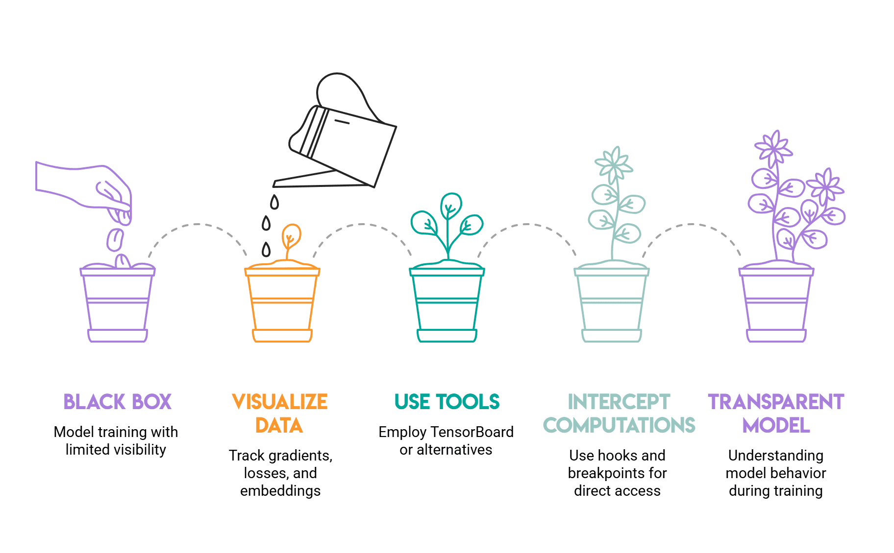
Visual Debugging Tools for Machine Learning: Essential Strategies for Model Transparency and Performance.

The intricate process of training a machine learning model often presents a paradox: the satisfaction of observing declining loss curves can abruptly halt when validation accuracy plateaus or loss metrics inexplicably spike. In these critical moments, the common reaction among practitioners is to resort to adding more logging or embarking on a trial-and-error hyperparameter tuning spree. However, a crucial step frequently overlooked is gaining genuine visibility into the internal workings of the model during its training phase. Visual debugging tools are increasingly recognized as indispensable instruments, offering profound insights that transform opaque model behavior into actionable diagnostic information.

This article delves into the critical role of visual debugging in modern machine learning workflows, exploring key aspects such as what to visualize during training (gradients, losses, and embeddings), the prominent tools facilitating these visualizations (TensorBoard and its primary alternatives), and advanced methods for directly capturing model computations using hooks and breakpoints. This systematic approach is vital for not only identifying issues but also understanding their underlying causes, thereby significantly accelerating model development and ensuring robust performance.

The Imperative for Model Transparency: Navigating the Black Box

The rapid advancement of deep learning has ushered in an era of unprecedented capabilities, yet it has simultaneously amplified the "black box" problem. Complex neural networks, with their millions or even billions of parameters, often operate in ways that defy intuitive understanding, making debugging a formidable challenge. Historically, machine learning debugging relied heavily on quantitative metrics and extensive log files, often leading to time-consuming trial-and-error processes. A 2022 survey by Algorithmia (now part of DataRobot) indicated that data scientists spend up to 40% of their time on tasks related to debugging and model maintenance, underscoring the significant overhead associated with identifying and resolving model performance issues. The advent of visual debugging tools represents a paradigm shift, moving from inferring problems from symptoms to directly observing the internal states and dynamics that dictate model behavior. This shift is particularly crucial as machine learning models transition from research curiosities to mission-critical components in diverse industries, where reliability, interpretability, and ethical considerations are paramount.

Core Visualizations for Diagnostic Clarity

Effective debugging hinges on observing the right metrics at the right time. Three primary categories of visualizations offer distinct yet complementary perspectives into a model’s learning process: loss curves, gradient magnitudes, and embedding spaces.

Visual Debugging Tools for Machine Learning Workflows

Illuminating Learning Trajectories: Loss Curves

The loss curve is arguably the most fundamental diagnostic plot in machine learning. It tracks the model’s error rate over epochs or training steps, providing an immediate snapshot of its learning progress. A healthy training process is typically characterized by both training and validation loss curves declining smoothly and remaining in close proximity, indicating effective learning without significant generalization issues.

However, deviations from this ideal pattern serve as critical diagnostic signals:

Overfitting: When the validation loss begins to rise while the training loss continues to fall, it’s a clear indication that the model is memorizing the training data rather than learning generalizable patterns. This divergence, often marked by a "red dotted line" in visualizations, signals the need for regularization techniques (e.g., dropout, L1/L2 regularization) or early stopping. Industry benchmarks suggest that severe overfitting can degrade model performance on unseen data by 20-50%.
Underfitting/Lack of Learning: If both training and validation loss curves plateau early and remain high, the model is failing to learn. This often points to fundamental issues such as an insufficient model capacity, incorrect learning rate (too high leading to instability, too low leading to sluggish convergence), or problems with the input data (e.g., noisy labels, insufficient feature representation).
Oscillating Loss: Erratic fluctuations in the loss curve, particularly during the initial stages, can suggest an overly aggressive learning rate, causing the model to overshoot optimal weight configurations.
Vanishing/Exploding Gradients (indirectly): While primarily observed through gradient visualizations, a very slow, smooth decrease in loss curves, especially in deeper networks, can indirectly suggest vanishing gradients preventing early layers from learning effectively. Conversely, wildly fluctuating loss can hint at exploding gradients.

Unveiling Learning Dynamics: Gradient Magnitudes

Gradients are the engine of neural network training, indicating the direction and magnitude of parameter updates. Visualizing gradient flow provides a direct window into the learning dynamics of each layer. The vanishing gradient problem, where gradients become infinitesimally small as they propagate backward through many layers, is a notorious challenge in deep learning, particularly prevalent in recurrent neural networks (RNNs) and very deep convolutional networks. This issue causes early layers to update their weights extremely slowly, effectively preventing them from learning meaningful representations.

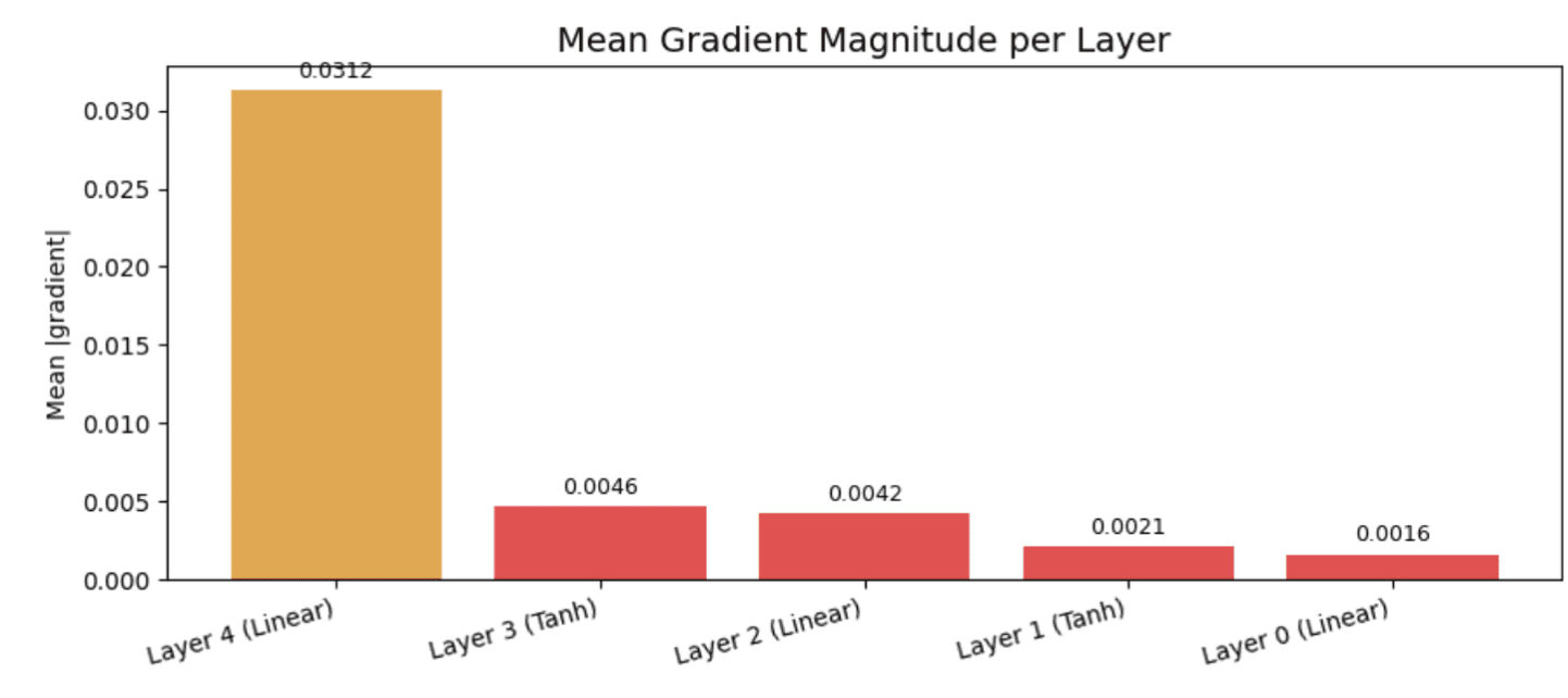
Consider a simple multi-layer perceptron. If the output layer receives a significant gradient (e.g., 0.031), but by the time it reaches the first layer, that magnitude has plummeted (e.g., to 0.0016), it signifies a dramatic reduction in learning signal. This 20-fold drop, as observed in a practical simulation, indicates that initial layers are "silently undertraining." Without visual inspection, this fundamental learning impediment might remain undetected for an entire training run, leading to suboptimal model performance.

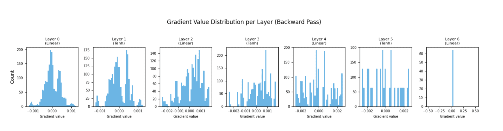
PyTorch’s register_backward_hook function offers a powerful mechanism to intercept gradient tensors during the backward pass without altering the model definition or training loop. By attaching a hook to each layer, practitioners can capture and plot gradient magnitudes or, more informatively, their complete distributions via histograms. A healthy network typically exhibits histograms across layers with roughly similar spreads. A narrow, spike-like distribution centered tightly around zero in early layers is a stark warning sign of vanishing gradients. Such visualizations allow for the early detection of these issues, often within the first few batches, enabling prompt architectural adjustments or hyperparameter tuning (e.g., using different activation functions like ReLU, incorporating Batch Normalization, or employing residual connections).

Decoding Learned Representations: Embeddings

When models transform raw inputs (like text or images) into learned, lower-dimensional representations known as embeddings, visualizing these spaces is crucial for understanding whether the model is effectively distinguishing between different concepts. The goal is to see data points belonging to the same class clustered together and clearly separated from other classes.

Dimensionality reduction techniques such as t-Distributed Stochastic Neighbor Embedding (t-SNE) and Uniform Manifold Approximation and Projection (UMAP) are commonly employed to project these high-dimensional embeddings into a 2D or 3D space for plotting. By coloring points according to their true class labels, practitioners can assess the quality of the learned representation. Well-separated, tight clusters indicate that the model has learned meaningful distinctions, laying a solid foundation for subsequent tasks like classification. Conversely, overlapping or scattered clusters suggest that the model has not yet grasped the underlying relationships in the data, potentially indicating issues with feature extraction, model architecture, or data quality. This debugging step is particularly valuable before adding the final classification layer, ensuring that the model’s core representation learning is robust.

The Ecosystem of Visual Debugging Tools

The demand for better model observability has fostered a rich ecosystem of tools, ranging from foundational frameworks to comprehensive MLOps platforms. These tools vary in their scope, integration, and target audience, but all aim to simplify the process of tracking, visualizing, and comparing machine learning experiments.

TensorBoard: The Pioneering Standard

TensorBoard, initially developed for TensorFlow, stands as the de facto starting point for many machine learning practitioners. Its integration with PyTorch via torch.utils.tensorboard has solidified its position across the broader deep learning community. TensorBoard offers robust capabilities for logging scalar values (loss, accuracy), visualizing histograms (weight and gradient distributions), displaying images, and an embedding projector for interactive exploration of high-dimensional representations. Its local deployment makes it accessible and straightforward for individual researchers and small teams. However, its primary limitation lies in its locality; sharing results within a distributed team often requires shared storage for log files or reliance on TensorBoard.dev, which has specific usage constraints. Despite this, its open-source nature and comprehensive feature set have made it an indispensable tool for countless projects, influencing the design of many subsequent platforms.

Weights & Biases (W&B): Collaboration and MLOps at Scale

Weights & Biases (W&B) has emerged as a leading solution for machine learning teams requiring robust collaboration features and detailed experiment tracking at scale. Its appeal stems from its cloud-first approach and comprehensive MLOps capabilities. With a simple two-line integration (wandb.init() and wandb.log()), W&B automatically syncs all experiment data—metrics, model checkpoints, system information, and configuration—to a centralized cloud dashboard. This facilitates seamless experiment comparison, allowing teams to analyze multiple runs grouped by project, quickly identifying the most effective hyperparameters or architectural changes.

W&B’s advanced features include built-in hyperparameter sweep visualization, which helps practitioners understand the impact of different parameters on model performance without manual analysis. It also automatically logs system metrics such as GPU utilization and memory usage, crucial for optimizing resource allocation. For teams managing a large volume of parallel experiments, W&B’s shared workspace significantly reduces the manual overhead of tracking and documenting findings, accelerating the iterative development cycle common in modern AI research and deployment. Its growing adoption reflects an industry trend towards integrated platforms that support the entire ML lifecycle, from experimentation to production monitoring.

Sacred: The Reproducibility Champion

Sacred takes a distinct philosophical approach, prioritizing reproducibility above all else. Instead of focusing solely on visualization, Sacred emphasizes creating an immutable record of every experiment. By annotating a training script with Sacred’s experiment decorator, the system automatically records the entire configuration, any runtime modifications, and all logged metrics into a persistent database (commonly MongoDB). This meticulous documentation ensures that any experiment from the past can be precisely reproduced, a critical capability for scientific rigor, auditing, and debugging complex models over time. While Sacred itself does not offer direct visualization, it pairs seamlessly with front-ends like Omniboard or Sacredboard, which provide graphical interfaces to explore the stored experiment data. This modularity adds a layer of complexity compared to integrated solutions like W&B but offers unparalleled auditability and control over experiment provenance, making it a favored choice in academic research and regulated industries.

Guild.ai: Non-Intrusive Experiment Management

Guild.ai caters to practitioners who prefer minimal modification to their existing training code. Operating primarily from the command line, Guild.ai allows users to execute training scripts via guild run train.py. It then automatically captures all logs, output files, and relevant metadata, linking them to a specific run. Metrics and run comparisons are accessible through Guild’s command-line interface (CLI) or its local UI. This non-intrusive approach makes Guild.ai an excellent choice when working with legacy codebases, third-party libraries, or complex frameworks where modifying the training loop might be cumbersome or undesirable. While it offers fewer advanced features than W&B, its low setup cost and emphasis on CLI-driven workflows make it a practical tool for many development environments.

Advanced Diagnostics: Hooks and Breakpoints

Beyond high-level dashboards and aggregated metrics, sometimes the most granular insights come from directly inspecting tensors at specific points within the neural network’s computation graph. PyTorch’s hook system and standard debugger breakpoints offer powerful, low-level mechanisms for this purpose.

Intercepting Computations: Forward and Backward Hooks

PyTorch’s hook system provides an elegant way to intercept and inspect tensors at any point during a model’s forward or backward pass without altering the model’s architecture.

register_forward_hook: This function attaches a callback to any module (layer). The callback fires every time the layer processes a batch, providing access to its input and output tensors. This is invaluable for tasks such as:
- NaN Detection: A forward hook can swiftly detect numerical instability by evaluating tensor.isnan().any() on the layer’s output, preventing the propagation of NaN values that can corrupt an entire training run. This can save hours of debugging by pinpointing the exact layer where instability originates.
- Feature Map Visualization: Hooks can capture intermediate feature maps, allowing for visualization of what the network "sees" at different depths, aiding in understanding representation learning.
- Custom Metric Calculation: Hooks enable the computation of layer-specific metrics that might not be directly exposed by standard training loops.
register_backward_hook: Similarly, this function provides access to the gradient tensors flowing backward through each layer. This is crucial for:
- Gradient Flow Analysis: As discussed earlier, visualizing gradient magnitudes or distributions per layer is a direct way to diagnose vanishing or exploding gradients.
- Gradient Clipping/Normalization: Hooks can be used to implement custom gradient manipulation techniques at a layer level.

Together, these hooks offer a highly flexible and non-invasive way to instrument a model, providing granular insights into its internal computations and quickly diagnosing issues related to numerical stability or gradient dynamics.

Interactive Inspection: Debugger Breakpoints

For immediate, step-by-step examination of model behavior, standard Python debuggers are indispensable. Dropping import pdb; pdb.set_trace() at any point in the code pauses execution and brings up an interactive prompt, allowing practitioners to inspect tensor shapes, verify data preprocessing outcomes, and manually step through the forward or backward pass. This is particularly useful during the initial stages of development or when integrating new components, ensuring that data flows as expected and intermediate tensor dimensions are correct.

Modern integrated development environments (IDEs) like VSCode and PyCharm enhance this experience by offering graphical breakpoint setting and dedicated panes for tensor inspection. This visual interface streamlines the debugging process, making it quicker and more intuitive than terminal-based pdb. Breakpoints are particularly valuable during the first few batches of a training run, serving as a critical checkpoint to confirm that the data pipeline, model architecture, and loss function are correctly configured before committing to a full, potentially lengthy, training cycle.

Broader Implications and Future Outlook

The proliferation and sophistication of visual debugging tools mark a significant maturation point for the machine learning field. Beyond merely identifying errors, these tools fundamentally transform the approach to model development, fostering a culture of transparency and systematic analysis rather than speculative guesswork.

Enhanced MLOps and Production Readiness: In an MLOps context, robust visual debugging capabilities are non-negotiable. They enable continuous monitoring of model health in production, quickly flagging performance degradations, data drift, or numerical instabilities before they impact end-users. This proactive stance leads to more reliable and resilient AI systems.

Accelerated Development Cycles and Cost Savings: By shortening the distance between identifying a symptom and understanding its root cause, visual debugging tools dramatically reduce the time spent on iterative experimentation and debugging. This translates directly into faster model development cycles and significant cost savings, especially for organizations running large-scale training jobs on expensive GPU clusters. A 2023 report by IBM estimated that effective MLOps practices, heavily reliant on monitoring and debugging tools, can reduce model deployment times by up to 75%.

Democratization of Complex Models: By providing intuitive visual feedback, these tools make complex deep learning architectures more accessible to a broader range of practitioners. Learners can gain a deeper understanding of how models learn, and experienced engineers can diagnose subtle issues more efficiently, lowering the barrier to entry for advanced AI development.

Ethical AI and Interpretability: The insights gleaned from visual debugging tools are also crucial for addressing ethical considerations in AI. By understanding how models arrive at decisions (e.g., through visualizing feature activations or embedding clusters), practitioners can identify and mitigate biases, ensure fairness, and develop more explainable AI systems. This aligns with the growing demand for XAI (Explainable AI) techniques that provide human-understandable explanations of model predictions.

While visual debugging tools cannot inherently "fix" a broken model, their profound contribution lies in providing the necessary instrumentation to understand why something is going wrong. They transform the once-opaque journey of model training into a series of observable, diagnosable events. As machine learning continues to evolve and its applications become ever more critical, the role of these tools in ensuring robust, reliable, and interpretable AI will only continue to grow, becoming an indispensable part of every data scientist’s toolkit.