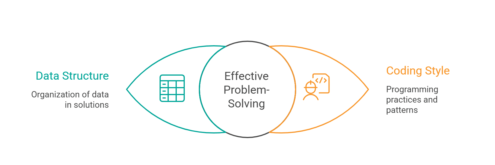
Visualizing Patterns in Solutions: How Dataset Shape Dictates Your Coding Style

The intricate structure of a dataset inherently guides the analytical and coding methodologies employed by data professionals, a phenomenon often observed intuitively but now quantifiable through systematic analysis. Whether grappling with time-series data, navigating complex star schemas, or manipulating multiple Pandas DataFrames, the underlying data architecture subtly yet powerfully directs the choice of functions, operators, and overall code organization. This principle, which posits that dataset "shape" is a primary determinant of coding style, has significant implications for efficiency, readability, and the reproducibility of data solutions across various platforms, including SQL and Python’s Pandas library.

The Unseen Hand: How Data Structure Shapes Solutions

Data problems, at their core, are not merely logical puzzles but rather a series of constraints imposed by the arrangement and relationships within tables. Understanding these constraints is paramount to developing effective and elegant solutions. The observed patterns reveal distinct archetypes of data structures that consistently lead to predictable coding styles.

Visualizing Patterns in Solutions: How Data Structure Affects Coding Style

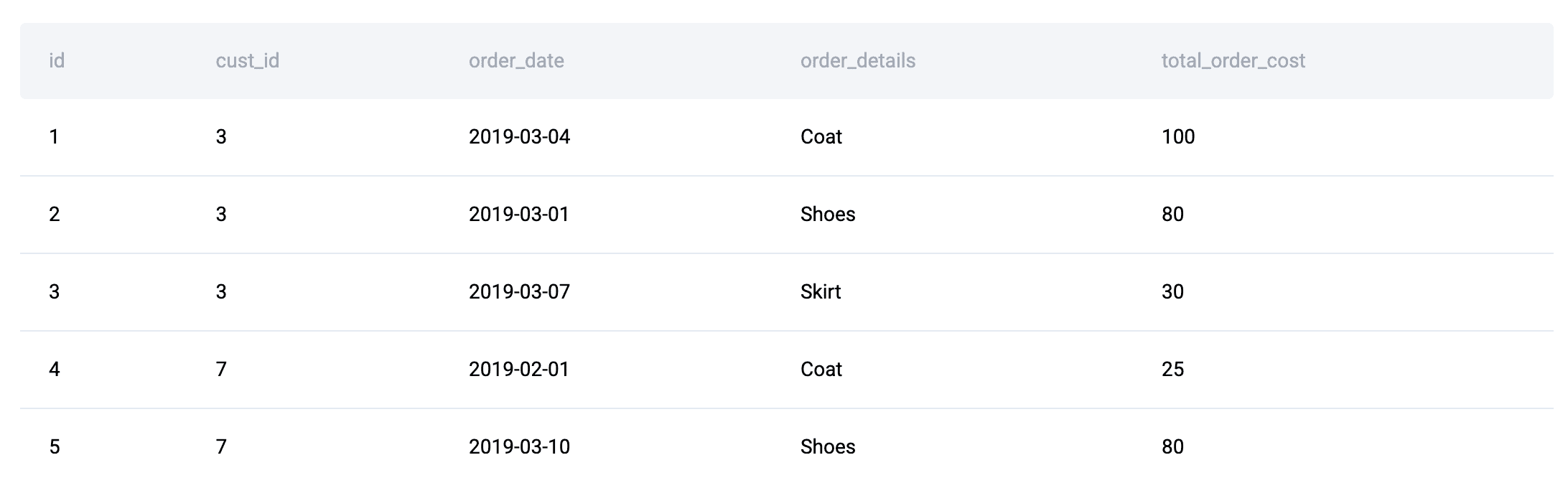
One prevalent archetype involves rows that depend on other rows, often encountered in temporal or sequential datasets. When a calculation for a given row necessitates information from adjacent rows – such as yesterday’s temperature, a previous transaction, or a running total – solutions naturally gravitate towards advanced analytical functions. In SQL, this translates to the frequent use of window functions like LAG(), LEAD(), ROW_NUMBER(), and DENSE_RANK(). For instance, a common interview scenario involves identifying the highest-cost orders per day, including ties. As illustrated by the "highest cost orders" problem from StrataScratch, a direct aggregation at the customer-day level is insufficient. The solution requires evaluating each customer’s daily total relative to others on the same date. This relative ranking, where the answer for one row is contingent on its peers within a specific partition (e.g., by order_date), mandates the application of window functions such as RANK() or DENSE_RANK(). These functions allow for partitioning data and ordering within those partitions, precisely addressing the need for row-dependent computations that simple GROUP BY clauses cannot achieve.

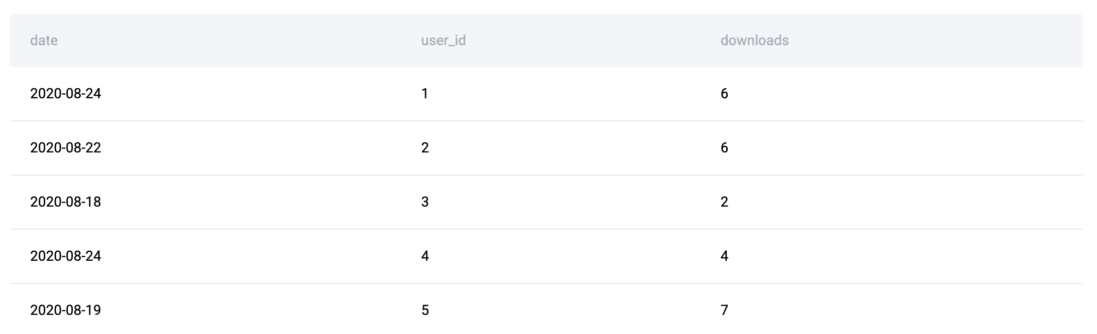
Another critical archetype emerges with multiple tables possessing distinct roles, typically seen in dimensional modeling where facts and dimensions are separated. Here, one set of tables describes entities (e.g., users, products), while another captures events or measurements (e.g., orders, downloads). Solutions to such problems almost invariably involve combining these disparate data sources before any meaningful aggregation can occur. In SQL, this manifests as extensive JOIN chains followed by GROUP BY operations. Pandas mirrors this pattern with .merge()and.groupby(). Consider the "Premium vs. Freemium" question, where user account statuses are in one table and download events in another. To analyze download patterns based on user subscription tiers, the entity attributes (user ID, account type) must first be linked with the event data (downloads) throughJOINclauses. Only after this integration can subsequent aggregation and analysis – like counting downloads per subscription type – take place. This fact-dimension pattern is foundational to business intelligence and reporting, makingJOINandGROUP BY` (or their Pandas equivalents) indispensable.

Finally, problems demanding small outputs based on exclusion logic often give rise to specific anti-join patterns. Questions like "who never did X" or "find entities without Y characteristic" typically require identifying records present in one set but absent in another. In SQL, this is commonly solved using LEFT JOIN ... IS NULL or NOT EXISTS subqueries. Pandas offers a vectorized approach with ~df['col'].isin(...), effectively filtering out rows where a column’s values are present in a specified list or series. This pattern is crucial for tasks such as identifying inactive users, detecting missing data points, or filtering out non-compliant entries.

Quantifying Coding Style: The Methodology

To transition from anecdotal observations to measurable insights, a systematic approach to extracting and quantifying specific code-structure traits is essential. This involves defining a limited set of observable features that reliably indicate how analysts interact with a dataset. While these features may not encompass all aspects of solution quality, they serve as robust signals of coding tendencies.

The study utilized a comprehensive set of educational questions from the StrataScratch platform, a repository of interview-style data problems, as its empirical foundation. By applying regular expression patterns to solution code, specific SQL and Pandas constructs were identified and counted.

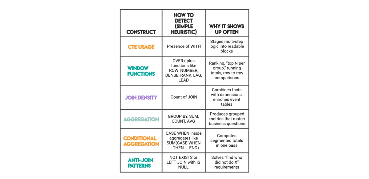
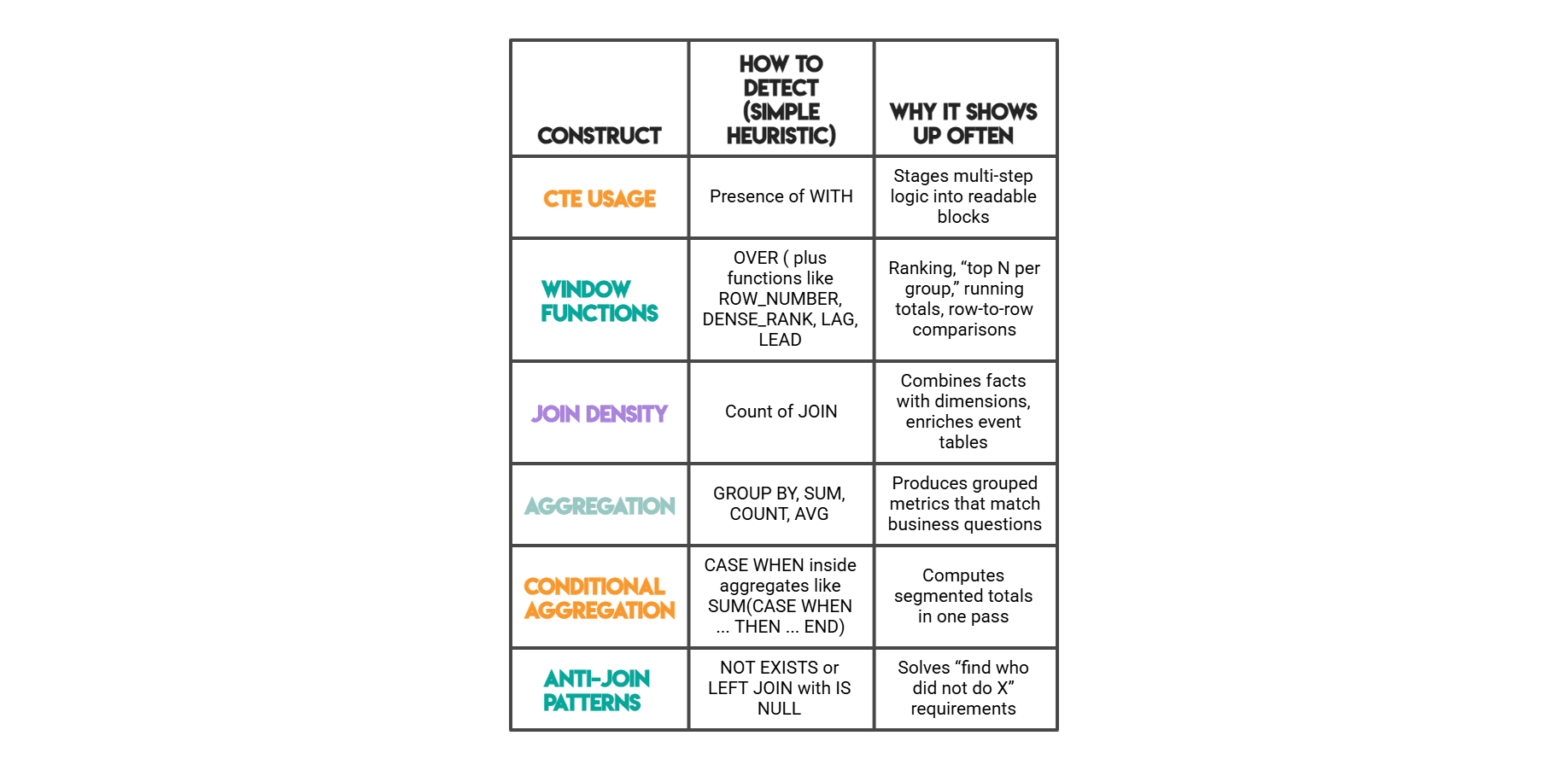
SQL Features Measured:

CTE (Common Table Expression): WITH keyword, indicating staged computation.
JOIN: JOIN keyword, signifying multi-table data integration.
GROUP BY: GROUP BY clause, denoting aggregation.
Window Function (OVER): OVER() clause, indicating row-dependent calculations.
DENSE_RANK: Specific window function for ranking with ties.
ROW_NUMBER: Specific window function for unique row numbering.
LAG: Window function for accessing previous row’s value.
LEAD: Window function for accessing next row’s value.
NOT EXISTS: Clause for exclusion logic.

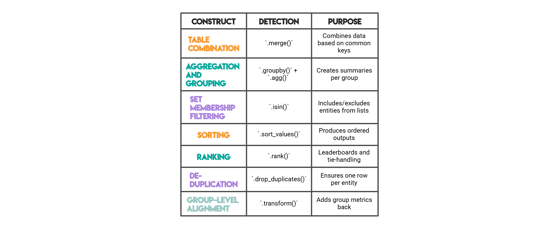
Pandas Features Measured:

.merge(): Method for combining DataFrames.
.groupby(): Method for aggregation.
.rank(): Method for ranking values.
.isin(): Method for checking membership.
.sort_values(): Method for sorting a DataFrame.
.drop_duplicates(): Method for removing duplicate rows.
.transform(): Method for applying a function element-wise to groups.

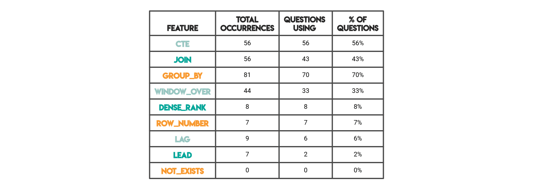
This methodology allowed for a consistent and reproducible comparison of coding styles across a vast array of problems. "Total occurrences" quantified the raw frequency of a pattern across all solutions, while "Questions using" indicated how many distinct problems featured at least one instance of that pattern, providing a measure of its prevalence in problem-solving.

Key Findings: Dominant Constructs in SQL and Pandas

The analysis of thousands of solutions on the StrataScratch platform yielded compelling insights into the most common coding constructs.

SQL Frequency Highlights:

Window Functions Surge in "Highest Per Day" and Tie-Friendly Ranking Tasks: The data unequivocally shows a high incidence of window functions, particularly RANK() and DENSE_RANK(), in problems requiring "highest per group" scenarios where ties must be preserved. For example, the "highest cost orders" problem, demanding the highest daily order cost per customer including ties, naturally leads to a solution utilizing RANK() OVER (PARTITION BY order_date ORDER BY total_daily_cost DESC). This two-step process—aggregate first, then rank within each partition—is a testament to the window function’s superiority over basic aggregation for such nuanced requirements. The ability to perform calculations across a set of table rows that are related to the current row, without collapsing rows, is invaluable for temporal analysis, cumulative sums, and comparative ranking.
CTE Usage Increases with Staged Computation: Common Table Expressions (CTEs) emerged as a cornerstone for solutions involving multiple computational stages. The WITH clause allows for breaking down complex queries into smaller, named, and more manageable logical units. This modularity significantly enhances readability, making it easier for analysts to understand the flow of data transformation and to debug intermediate results. Industry best practices advocate for CTEs as a means to improve query organization, mirroring software engineering principles of decomposition and abstraction. Problems that mix filtering, joining, and complex metric calculations often benefit immensely from this staged approach, preventing monolithic and difficult-to-maintain queries.
JOIN Plus Aggregation as the Default for Multi-Table Business Metrics: Unsurprisingly, when business metrics span multiple tables—with measures residing in one table and descriptive dimensions in another—JOIN clauses followed by GROUP BY operations become the default solution pattern. This reflects the fundamental nature of analytical queries in relational databases. Once data from various sources is combined via JOINs, GROUP BY provides the mechanism to summarize and aggregate information at the desired level of granularity, often employing conditional totals using SUM(CASE WHEN ... THEN ... END) for specific metric calculations. This pattern is the backbone of most data warehousing and reporting systems.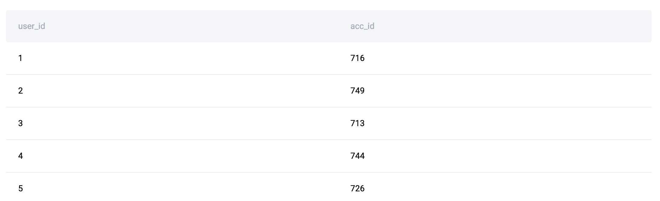

Pandas Method Highlights:

.merge() Appears Whenever the Answer Depends on More Than One Table: Similar to SQL’s JOIN, Pandas’ .merge() method is omnipresent in solutions where data integration from multiple DataFrames is required. The "City with Most Customers" problem, for instance, involves combining order data with payment information. The initial step is to merge() these DataFrames based on a common key like order_id. This initial data combination is crucial, as subsequent filtering, grouping, and comparison steps—like identifying the city with the maximum number of orders after filtering by date and promo code status—are significantly simplified once all relevant data resides in a single DataFrame. The prevalence of .merge() underscores the reality that real-world data rarely resides in a single, perfectly structured table.
.groupby() is a Core Operation for Aggregation: Following .merge(), .groupby() is consistently a top-used Pandas function, reflecting its fundamental role in data aggregation and summarization. Whether calculating sums, averages, counts, or applying custom aggregation functions, .groupby() is the workhorse for deriving insights from grouped data.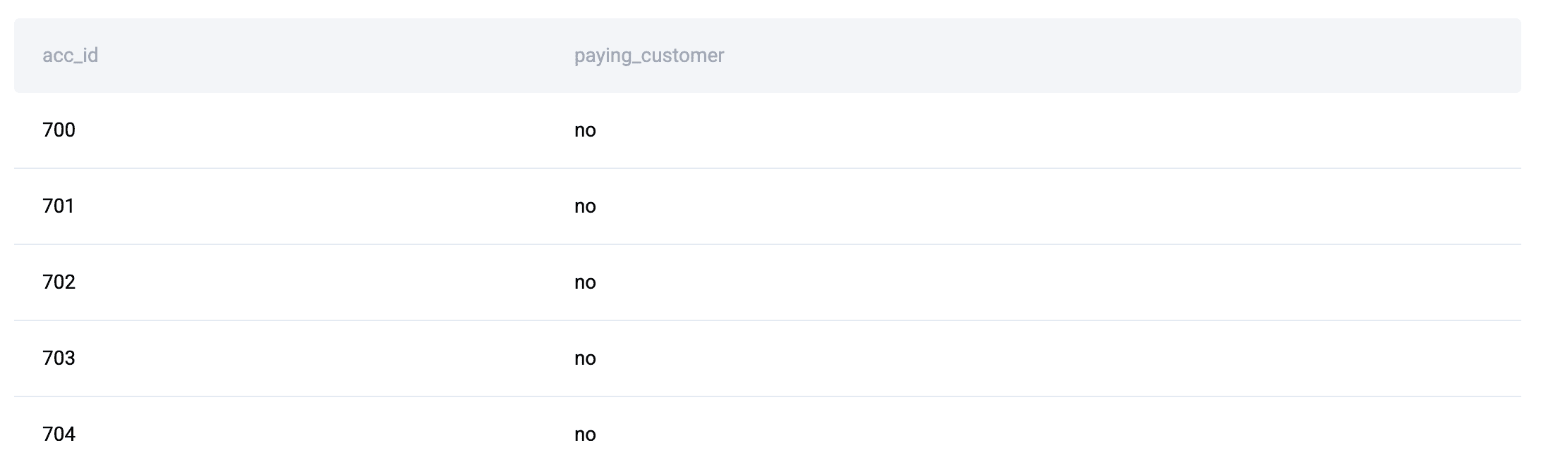

The Enduring Rationale: Why These Patterns Persist

The consistent emergence of these coding patterns is not accidental; it is deeply rooted in the inherent characteristics of data and the analytical tasks required.

Time-based Tables Often Call for Window Logic: Data with a temporal component inherently demands ordered logic. Problems involving comparisons between periods, running totals, cumulative sums, or selecting the "highest/lowest per day/month" necessitate the context of preceding or succeeding rows. Window functions are purpose-built for these scenarios, allowing computations over a defined "window" of rows related to the current row. This capability is critical for time-series analysis, trend identification, and event sequencing, especially when preserving ties in ranking is a business requirement.
Multi-step Business Rules Benefit from Staging: Complex business problems frequently involve a sequence of data transformations and calculations. Attempting to condense all logic into a single, monolithic query or function can lead to unreadable, unmanageable, and error-prone code. Staging computations, whether through SQL CTEs or intermediate Pandas DataFrames, provides clarity, simplifies debugging, and enhances maintainability. This modular approach aligns with the principle of "divide and conquer," making complex analytical tasks more approachable and verifiable at each step.
Multi-Table Questions Naturally Increase Join Density: The normalization of relational databases, a cornerstone of good database design, dictates that data is often distributed across multiple tables to reduce redundancy and improve data integrity. Consequently, deriving comprehensive metrics or insights often requires reassembling this distributed information. If a metric depends on attributes stored in a different table, JOIN operations are not merely an option but a necessity. The more fragmented the data, the higher the "join density" will be in the resulting solution. Once tables are combined, grouped summaries become the natural next analytical step to synthesize the integrated data.

Practical Takeaways for Faster, Cleaner Solutions

Recognizing these structural patterns early in the problem-solving process can dramatically improve a data professional’s efficiency and the quality of their solutions.

Anticipate the Framework: Instead of immediately diving into syntax, begin by analyzing the dataset’s shape and the nature of the question. Is it a time-series problem requiring row-dependent calculations? A multi-source integration task? An exclusion query? Anticipating the dominant construct (e.g., window functions, JOIN + GROUP BY, anti-joins) provides a foundational framework for the solution.
Embrace Modularity: For complex problems, consciously break down the solution into logical stages. Utilize SQL CTEs or intermediate Pandas DataFrames. This approach not only makes the code more readable and easier to debug but also allows for independent validation of each step, minimizing errors.
Master Core Constructs: Invest time in deeply understanding the fundamental functions and methods that address these common data patterns. For SQL, this includes JOIN types, GROUP BY with aggregate functions, and the full suite of window functions. For Pandas, proficiency in .merge(), .groupby(), .apply(), and vectorized operations like .isin() is crucial.
Practice Pattern Recognition: Actively seek out and classify new data problems based on their underlying structure. This deliberate practice will refine intuition, enabling quicker identification of appropriate solution patterns and reducing the time spent on trial-and-error.

Conclusion

The evidence strongly suggests that coding style is not merely a matter of personal preference but a direct consequence of dataset structure. Time-based problems and "highest per group" questions consistently lead to the use of window functions. Multi-step business rules inherently benefit from the modularity offered by CTEs. Furthermore, metrics spanning multiple tables inevitably increase JOIN density, a pattern faithfully mirrored by Pandas’ .merge() and .groupby() operations.

This profound connection means that a shift in mindset is invaluable for data practitioners. Rather than approaching each problem as a blank slate or relying solely on memorized tricks, one can reason from the data itself. By asking: "Is this a per-group maximum? A staged business rule? A multi-table metric?", data professionals can predict the dominant coding construct even before writing a single line of code. This anticipatory approach leads to faster solution drafting, simpler validation, and greater consistency across diverse problems and platforms. Ultimately, mastering the art of recognizing dataset shape allows for the efficient and elegant crafting of data solutions, transforming complex analytical challenges into structured, manageable tasks.

Nate Rosidi is a data scientist and in product strategy. He’s also an adjunct professor teaching analytics, and is the founder of StrataScratch, a platform helping data scientists prepare for their interviews with real interview questions from top companies. Nate writes on the latest trends in the career market, gives interview advice, shares data science projects, and covers everything SQL.