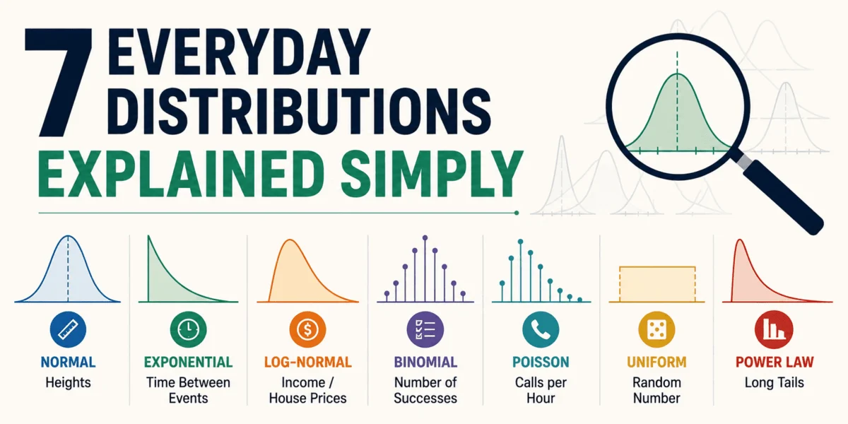
Unlocking the Language of Data: Seven Everyday Statistical Distributions Explained

In an increasingly data-driven world, understanding the fundamental patterns that govern numerical observations is no longer the sole domain of statisticians; it is a critical skill for anyone seeking to interpret reality. While many have heard the phrase "that’s a normal distribution" as a catch-all explanation, the truth is that data tells many different stories, each with its own unique shape and implications. These "stories" are known as statistical distributions, and they describe how numbers tend to appear in real-life scenarios—some are smooth curves, some are lumpy, and some reflect outcomes as simple as a coin flip.

This article provides an accessible, everyday exploration of seven key statistical distributions that, once recognized, transform abstract concepts into practical insights. Without delving into heavy mathematical formulas, this guide aims to illuminate the "vibe" of each distribution, empowering readers to see patterns in everything from daily routines to global phenomena. Spotting these patterns shifts statistics from an academic subject to a powerful "cheat code" for interpreting the world, enabling more informed decisions and a deeper understanding of underlying processes.

The Foundational Bell: Normal Distribution

The normal distribution, often visualized as the iconic bell curve, is arguably the most recognized statistical pattern. It emerges when a variable is influenced by a multitude of small, independent factors that collectively nudge its value up or down. Imagine a scenario where numerous minor forces contribute to a final outcome; the result tends to cluster around an average value, with extreme deviations becoming progressively rarer. This phenomenon is precisely what the Central Limit Theorem elucidates: the distribution of sample means of a large number of independent, identically distributed variables will be approximately normal, regardless of the underlying distribution of the original variables.

Historically, the normal distribution was first described by Abraham de Moivre in 1733, later popularized by Carl Friedrich Gauss and Pierre-Simon Laplace for modeling errors in astronomical observations. Its prevalence in natural and social sciences stems from its ability to model continuous data where values concentrate around a central mean. Key parameters defining a normal distribution are its mean (µ), which dictates the center of the curve, and its standard deviation (σ), which measures the spread or dispersion of the data. A smaller standard deviation indicates data points are tightly clustered around the mean, while a larger one suggests greater variability.

Real-world examples are ubiquitous:

Human Heights: Within a specific age group and population, individual heights tend to follow a normal distribution, with most people falling near the average height and fewer individuals being exceptionally tall or short.
Measurement Errors: In scientific experiments or manufacturing, small, random errors often accumulate to form a normal distribution around the true value. For instance, the slight inaccuracies in a machine cutting parts to a specified length.
Test Scores: In large, diverse groups, standardized test scores frequently approximate a normal distribution, reflecting a natural range of abilities with most students performing around the average.
Stable Processes: The time an average person takes to answer an email on a typically stable day might be normally distributed, with most responses falling within a consistent window and occasional outliers.

The symmetry of the normal distribution is a defining characteristic. Values are concentrated at the center, and the frequency of values decreases symmetrically as one moves further from the mean. Phrases like "two standard deviations away" quantify how unusual an observation is, with values beyond two standard deviations from the mean occurring in roughly 5% of cases, and beyond three standard deviations in less than 1%. Statisticians, while acknowledging its widespread applicability, caution against assuming normality without empirical validation, as misapplying it can lead to erroneous conclusions. Nevertheless, its role in hypothesis testing, quality control, and risk assessment remains foundational in numerous disciplines, from finance to public health.

The Level Playing Field: Uniform Distribution

In stark contrast to the bell curve, the uniform distribution is the embodiment of impartiality. It describes a scenario where every outcome within a defined range has an exactly equal probability of occurring. This "no favorites" pattern makes it a crucial baseline for understanding true randomness and for constructing simulations where unbiased outcomes are desired.

The uniform distribution comes in two primary forms:

Discrete Uniform Distribution: Applies to a finite number of distinct outcomes, each with the same probability. For example, rolling a fair six-sided die, where each face (1, 2, 3, 4, 5, 6) has a 1/6 chance of appearing.
Continuous Uniform Distribution: Applies to a continuous range of values, where any value within that range is equally likely. For instance, generating a random number between 0 and 1, where every fractional value within that interval has the same likelihood of being selected.

Perfect examples are often human-engineered or idealized:

Fair Dice and Cards: Rolling a fair die or drawing a card from a well-shuffled deck are classic discrete uniform examples.
Random Number Generators: Computer algorithms designed to generate random numbers (often between 0 and 1) typically aim for a continuous uniform distribution, forming the bedrock of simulations and cryptographic processes.
Equal-Slice Prize Wheels: A physical prize wheel with equally sized segments, when spun fairly, represents a discrete uniform distribution for the prizes.
Sampling: In statistics, random sampling often relies on uniform distribution principles to ensure every member of a population has an equal chance of selection.

In the natural world, true uniform distributions are rare because underlying biases, external factors, or inherent mechanisms usually skew outcomes. However, its theoretical purity makes it invaluable as a model. When simulating complex systems, performing Monte Carlo experiments, or establishing a null hypothesis for random behavior, the uniform distribution serves as the clean "starting point." Its importance in computational statistics cannot be overstated, providing the foundation for generating pseudo-random numbers that underpin everything from video games to scientific research.

Counting Successes: The Binomial Distribution

When an experiment involves a fixed number of independent trials, each yielding one of two possible outcomes—often termed "success" or "failure"—the binomial distribution steps in to answer the question: "How many successes can we expect?" It’s a fundamental concept in probability that quantifies the number of successes in a series of Bernoulli trials.

The binomial distribution is characterized by four key conditions:

Fixed Number of Trials (n): The experiment consists of a predetermined count of repetitions.
Two Possible Outcomes: Each trial results in either a "success" or a "failure."
Independent Trials: The outcome of one trial does not influence the outcome of any other trial.
Constant Probability of Success (p): The probability of success remains the same for every trial.

With these conditions met, the binomial distribution allows for the calculation of the probability of observing a specific number of successes (k) out of n trials.

Everyday applications are widespread:

Marketing Campaigns: If an email campaign is sent to 100 recipients (n=100) and the historical open rate is 20% (p=0.2), the binomial distribution can predict the probability of 15, 20, or 25 people opening the email.
Sports Performance: A basketball player attempting 20 free throws (n=20) with a historical success rate of 75% (p=0.75) can have the probability of making 10, 15, or all 20 shots estimated using this distribution.
Quality Control: In manufacturing, if 50 items are sampled from a production line (n=50) and the defect rate is known to be 2% (p=0.02), the binomial distribution helps determine the likelihood of finding 0, 1, or 2 defective items.
Medical Trials: Clinical trials often involve patients responding to a treatment (success) or not (failure) over a fixed number of participants, making binomial analysis crucial for assessing drug efficacy.

The binomial distribution is the mathematical backbone of "conversion rate" thinking. When a business analyst states, "Our website signup rate is 8%," the binomial distribution is implicitly providing the framework for understanding expected variation. It allows for the computation of confidence intervals around observed rates and helps identify when an observed number of successes is statistically significant or merely due to random chance, thereby informing decisions in A/B testing, product development, and operational efficiency.

Events Over Time and Space: The Poisson Distribution

When the focus shifts from a fixed number of trials to counting the occurrences of discrete events within a continuous interval of time or space, the Poisson distribution becomes the tool of choice. It models the number of events happening independently and randomly at a constant average rate, particularly useful for relatively rare events.

Named after French mathematician Siméon Denis Poisson, who introduced it in 1838, this distribution is characterized by a single parameter, lambda (λ), which represents the average number of events expected in a given interval. A key assumption of the Poisson distribution is that the events occur independently and that the rate of occurrence is constant over the interval. It often serves as an approximation to the binomial distribution when the number of trials (n) is large and the probability of success (p) is small.

Diverse applications include:

Customer Service: The number of customer support tickets received per hour at a call center (e.g., an average of 10 tickets per hour).
Quality Assurance: The number of typos per page in a long document, or the number of defects per square meter of fabric.
Traffic Management: The number of cars passing a specific checkpoint in a 5-minute interval during off-peak hours.
Website Analytics: Daily website signups or page views, assuming traffic is relatively stable and arrivals are independent.
Epidemiology: The number of new cases of a rare disease in a population over a specific period.
Reliability Engineering: The number of component failures in a complex system within a given operational window.

The Poisson distribution has a unique "vibe" focused on counts within a window, rather than binary outcomes. It helps answer "how many happened?" not "did it happen?" Its predictive power in modeling seemingly messy, random event counts has made it indispensable in fields like queuing theory, risk management, public health surveillance, and inventory control. Experts highlight its utility in predicting the likelihood of various event counts, allowing businesses and organizations to plan resources effectively, from staffing call centers to managing critical infrastructure maintenance schedules.

The Waiting Game: Exponential Distribution

Closely related to the Poisson distribution, the exponential distribution addresses a different, yet complementary, question: "How long will it be until the next event occurs?" While Poisson counts the number of events in a fixed interval, the exponential distribution models the waiting time between these events in a Poisson process. It is a continuous probability distribution and possesses a unique characteristic known as the "memoryless" property. This property implies that the probability of an event occurring in the future is independent of how much time has already passed without the event occurring. In simpler terms, if a light bulb has an exponentially distributed lifespan, its remaining useful life doesn’t change regardless of how long it has already been working.

The exponential distribution is also characterized by a single parameter, λ (lambda), which is the rate parameter (the average number of events per unit of time, inverse of the average waiting time). A higher λ means events occur more frequently, leading to shorter waiting times.

Practical examples abound:

Customer Arrivals: The time until the next customer walks into a quiet shop or arrives at a service counter. If customers arrive at an average rate of 5 per hour, the exponential distribution can model the probability of waiting 10, 20, or 30 minutes for the next arrival.
System Failures: The time between random system failures in simplified reliability setups, such as the lifespan of certain electronic components before they fail.
Call Center Queues: The duration a caller waits in a queue before being connected to an agent, assuming calls arrive randomly.
Natural Phenomena: The time between earthquakes in a specific region, or the time between successive radioactive decays of an atom.

The memoryless property of the exponential distribution can feel counter-intuitive to human experience, which often seeks patterns and assumes that an overdue event is "more likely" to happen soon. However, for truly random processes with a constant underlying rate, the past does not influence the future. This makes the exponential distribution invaluable in operational research, reliability engineering, and queuing theory for designing efficient systems, optimizing service levels, and performing predictive maintenance, especially for components that do not exhibit "wear and tear" in a traditional sense.

The Skewed Reality: Lognormal Distribution

The lognormal distribution emerges in scenarios where a variable is the product of many independent factors, rather than their sum. If the logarithm of a variable is normally distributed, then the variable itself follows a lognormal distribution. This often results in a distribution that is positively skewed, meaning it has a long "right tail" where a few values are extremely large, while the majority of values are clustered towards the lower end.

This distribution is prevalent in fields where growth and multiplicative effects are significant. Unlike the normal distribution, which is symmetric around its mean, the lognormal is asymmetrical. Its mean is typically higher than its median, reflecting the disproportionate influence of those few extremely large values.

Common applications include:

Income and Wealth Distribution: In many economies, a small percentage of the population holds a disproportionately large share of wealth, leading to a highly right-skewed distribution of income and assets.
Real Estate Prices: Home prices in many markets often follow a lognormal pattern, with a large number of moderately priced homes and a smaller number of extremely expensive properties.
Project Completion Times: The time required to complete complex projects, where numerous interdependent tasks multiply to determine the final duration, often exhibits a lognormal distribution.
Biological Measurements: The size of living organisms (e.g., bacteria, fish), or the concentration of certain substances in biological systems, frequently conforms to a lognormal pattern due to multiplicative growth processes.
Financial Markets: Stock prices and asset returns over periods longer than a day often approximate a lognormal distribution, reflecting compounding growth.

The lognormal distribution highlights why "average" can be a misleading metric. In a lognormal dataset, a few exceptionally high values can significantly inflate the arithmetic mean, making it unrepresentative of the typical value. In such contexts, the median (the middle value) often provides a more honest and insightful representation of the central tendency. Understanding the lognormal distribution is crucial for accurate financial modeling, assessing economic inequality, and interpreting data in environmental science and biology, guiding researchers to use appropriate statistical measures and avoid misinterpretations.

The Giants and the Smalls: Power Law Distribution

An even more extreme form of long-tailed behavior than the lognormal distribution is the power law distribution. It describes phenomena where a small number of entities possess a disproportionately large share of a characteristic, while the vast majority possess very little. This "fat tail" means that extremely large events, though rare, are far more common than would be predicted by a normal or even lognormal distribution. Power laws are scale-free, meaning their shape looks the same regardless of the scale at which they are viewed.

Historically, the observation of such distributions dates back to Vilfredo Pareto’s work on income distribution in 1896, where he noted that roughly 80% of the wealth was owned by 20% of the population – the famous Pareto principle. Later, George Kingsley Zipf observed similar patterns in word frequencies (Zipf’s Law), where a few words are used very frequently, and many words are used rarely. These distributions often arise in complex systems where "preferential attachment" or "rich-get-richer" dynamics are at play.

Observable in numerous complex systems:

City Sizes: A few mega-cities contain vast populations, while the majority of settlements are small towns and villages.
Social Media Followers: A handful of influencers or celebrities have millions of followers, while most users have a modest number.
Website Traffic by Page: A small number of "pillar" pages or popular articles receive the vast majority of a website’s traffic.
Sales by Product: A few "blockbuster" products account for a large percentage of total sales, with many niche products selling far less.
Scientific Citations: A small number of highly influential papers accumulate a disproportionate number of citations.
Earthquake Magnitudes: While small earthquakes are frequent, large, destructive earthquakes are rare but occur with a frequency that follows a power law, not a normal distribution.

The power law distribution has profound implications for understanding inequality, resilience of networks, and critical phenomena. It suggests that interventions aimed at the "average" may miss the true drivers of a system. For instance, in social networks, targeting the highly connected "hubs" (the giants) can have a much greater impact than targeting the average user. Furthermore, its presence in natural systems, such as the clustering of matter in the universe (setting aside complex gravitational dynamics and cosmic expansion, which introduce other factors), underscores that significant heterogeneity and extreme outcomes are fundamental aspects of many complex phenomena. Experts in complex systems emphasize that recognizing power laws is crucial for designing robust networks, understanding market dynamics, and predicting the behavior of systems where extreme events play a dominant role.

Conclusion: Beyond the Formulas – Mastering Data Intuition

The journey through these seven statistical distributions reveals that data is never merely a collection of numbers; it is a narrative waiting to be understood. From the symmetric clustering of the normal curve to the extreme imbalances of a power law, each distribution tells a unique story about how phenomena unfold in the real world. The true power lies not in memorizing complex formulas, but in developing an intuitive "pattern recognition" ability that allows one to identify the underlying distribution shaping a dataset.

This statistical intuition, akin to having "receipts" for observed patterns, empowers individuals to critically assess information and make more informed judgments. Whether analyzing personal inbox behavior, interpreting economic trends, or evaluating the efficacy of a marketing campaign, recognizing these fundamental patterns provides a sharper sense of what constitutes normal variation, pure randomness, or a signal truly worthy of investigation. In an era deluged with information, the ability to discern these underlying statistical narratives transforms data from an overwhelming torrent into a decipherable guide for navigating and interpreting the complexities of our world.

Nahla Davies is a software developer and tech writer whose expertise spans across various domains of technology. Prior to dedicating her work full time to technical writing, Ms. Davies served as a lead programmer at an Inc. 5,000 experiential branding organization, contributing to projects for high-profile clients including Samsung, Time Warner, Netflix, and Sony, among other notable industry leaders. Her practical experience in software development and her ability to articulate complex technical concepts make her a respected voice in the technology landscape.