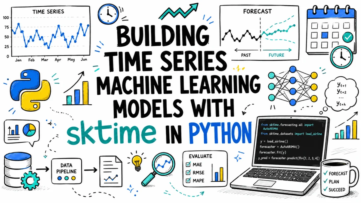
The landscape of machine learning has seen significant evolution, yet specialized tools for time series data have long presented a challenge, often forcing practitioners to adapt general-purpose libraries. A notable development in this space is sktime, a Python library engineered to bridge this gap by providing a scikit-learn-compatible API specifically for temporal data. This framework facilitates a wide array of time series tasks, including forecasting, classification, regression, and clustering, all while maintaining a consistent and intuitive interface. Its emergence streamlines complex workflows, making advanced time series analytics more accessible and efficient for data scientists and engineers.
The Intricacies of Time Series Data and the Need for Specialization
Time series data, characterized by sequential measurements taken over time, is ubiquitous across industries. From sensor readings in industrial Internet of Things (IoT) deployments to server metrics in cloud infrastructure, financial market data, and patient vital signs in healthcare, its unique structure demands specialized analytical approaches. Unlike conventional tabular datasets, where individual rows are often assumed to be independent, time series data exhibits inherent temporal dependencies. Future values are intrinsically linked to past observations, and critical patterns like seasonality (repeating patterns over fixed periods), trend (long-term increase or decrease), and autocorrelation (correlation of a series with its lagged versions) are fundamental to its interpretation and prediction.
Traditional machine learning libraries, such as scikit-learn, are primarily designed for static, tabular datasets where observations are independent and identically distributed (i.i.d.). Attempting to apply these tools directly to time series data often leads to suboptimal models, erroneous predictions, and the potential for data leakage. The explicit ordering of data points, the non-stationarity introduced by trends and seasonality, and the need for specialized preprocessing steps (e.g., detrending, deseasonalizing, imputation tailored for temporal gaps) highlight the limitations of general-purpose frameworks in this domain. Prior to sktime, practitioners frequently resorted to bespoke code, combining elements from libraries like statsmodels or pmdarima with custom scikit-learn wrappers, a process that was often cumbersome and prone to inconsistencies.
sktime: A Unified and Extensible Framework
sktime addresses these challenges by offering a cohesive ecosystem designed from the ground up for time series analysis. Its core philosophy revolves around extending the familiar scikit-learn API – featuring fit, predict, and transform methods – to explicitly handle the temporal dimension. This design choice significantly reduces the learning curve for data scientists already proficient in scikit-learn, while providing the necessary abstractions for time series specific operations.
The library supports diverse time series data structures, categorized to reflect varying complexities:
- Series: Representing a single time series, typically a
pandas.Seriesorpandas.DataFramewhere each row is a time-indexed observation. This is commonly used in univariate forecasting tasks. - Panel: A collection of multiple independent time series, often stored as a
pandas.DataFramewith a 2-levelMultiIndexto distinguish between different series. This is crucial for problems involving multiple related or unrelated time series. - Hierarchical: A structured set of time series with aggregation levels across multiple dimensions, using a
pandas.DataFramewith a 3+ levelMultiIndex. This caters to more complex scenarios where data exists at various granularities and aggregation levels (e.g., sales data by product, store, and region).
Crucially, sktime supports various time indexes, including DatetimeIndex, PeriodIndex, Int64Index, and RangeIndex, provided they are monotonic. For DatetimeIndex, the freq attribute is essential for correct temporal interpretation.
A Practical Demonstration: Forecasting Industrial HVAC Temperatures
To illustrate sktime‘s capabilities, a common industrial application – forecasting temperature readings from an HVAC sensor – provides a compelling example. Such a scenario is vital for energy management, predictive maintenance of equipment, and maintaining optimal environmental conditions in facilities.
Simulating Real-World Sensor Data
The demonstration begins by generating a synthetic dataset that closely mimics real-world sensor behavior over 90 days with hourly readings, starting January 1, 2026. This dataset is engineered to incorporate several realistic characteristics:
- Trend: A gradual upward trend of 5 degrees Celsius over the 90-day period, simulating environmental changes like the onset of summer or gradual system degradation.
- Daily Seasonality: A pronounced daily cycle where temperatures peak around 2 PM and dip around 4 AM, reflecting typical human activity patterns or operational schedules within a factory setting. This sinusoidal pattern is a classic feature in many natural and artificial systems.
- Noise: Random fluctuations introduced through Gaussian noise, representing measurement inaccuracies, minor environmental disturbances, or unmodeled factors.
- Missing Values: Deliberate introduction of
np.nanvalues at specific points, simulating sensor dropouts or data transmission errors, a common occurrence in industrial IoT.
The resulting pandas.Series, y, named "temp_celsius," encapsulates these complexities, providing a robust testbed for sktime‘s preprocessing and forecasting capabilities. The data, spanning 2160 hourly observations, clearly demonstrates the presence of missing values and a time-aware index with a defined frequency.
Chronological Data Splitting and Forecasting Horizon
A fundamental difference in time series analysis compared to traditional machine learning is the methodology for splitting data into training and testing sets. Random shuffling, a common practice in tabular data, is strictly forbidden in time series to prevent data leakage, where future information inadvertently influences the training process. sktime provides temporal_train_test_split, a dedicated utility that ensures a clean chronological division. In this example, the last 7 days (168 hours) of data are reserved as the test set, allowing the model to be trained on past observations and evaluated on unseen future data.
Defining the ForecastingHorizon is equally critical. This specifies the exact time steps for which predictions are desired. sktime‘s ForecastingHorizon object can handle both relative (e.g., "predict 1, 2, 3 steps ahead") and absolute (e.g., "predict for specific timestamps") horizons. For the HVAC example, an absolute horizon corresponding to the y_test.index is used, ensuring predictions align precisely with the held-out test period.
Building Robust Forecasting Pipelines with TransformedTargetForecaster
Real-world sensor data necessitates robust preprocessing. Missing values must be handled, and underlying patterns like trend and seasonality often need to be isolated or removed to enable forecasters to model the stationary residuals effectively. sktime‘s TransformedTargetForecaster is a powerful composition tool that allows chaining multiple transformations with a forecaster into a single, coherent pipeline. This mimics scikit-learn‘s Pipeline but is specifically designed for time series, ensuring transformations are applied to the target series before fitting and automatically reversed during prediction.
The proposed pipeline for the HVAC temperature forecast comprises four sequential steps:
- Imputation:
Imputer(method="linear")addresses missing sensor readings by employing linear interpolation, a suitable method for filling gaps in sequential data. - Detrending:
Detrender()removes the underlying linear trend from the series, ensuring that the subsequent forecaster operates on a more stationary dataset, which often improves model performance. - Deseasonalization:
Deseasonalizer(model="additive", sp=24)extracts the daily seasonality. Thesp=24parameter explicitly indicates a seasonal period of 24 hours, crucial for hourly data. This step isolates the core, deseasonalized component of the series. - Forecasting:
ExponentialSmoothing(trend=None, seasonal=None)is then applied to the cleaned, stationary residuals. By settingtrend=Noneandseasonal=None, the Exponential Smoothing model focuses solely on the remaining irregular component, leveraging the prior detrending and deseasonalization steps.
This pipeline is fitted to the training data, and predictions are generated for the defined forecasting horizon. The output reveals the model’s initial forecasts for the test period.
Evaluating Forecast Accuracy
Assessing the performance of a time series model requires appropriate metrics. sktime integrates seamlessly with standard evaluation metrics tailored for forecasting. Mean Absolute Error (MAE) and Mean Absolute Percentage Error (MAPE) are widely adopted for their interpretability. MAE provides the average magnitude of errors in the same units as the forecast variable (degrees Celsius in this case), while MAPE expresses error as a percentage, useful for comparing accuracy across different scales. For the Exponential Smoothing pipeline, an MAE of approximately 0.584 °C and a MAPE of 2.40% indicate a reasonably accurate forecast for the industrial temperature data.
Model Agnosticism: Swapping Forecasters with Ease
One of sktime‘s most significant advantages is its modularity. The TransformedTargetForecaster architecture allows for effortless swapping of the underlying forecasting algorithm without altering the preprocessing steps. This facilitates rapid experimentation and comparison of different models. Replacing ExponentialSmoothing with an ARIMA model (ARIMA(order=(1, 1, 1), suppress_warnings=True)) within the same preprocessing pipeline demonstrates this flexibility. The ARIMA model, applied to the already detrended and deseasonalized residuals, yields comparable performance (MAE of 0.586 °C, MAPE of 2.41%), underscoring the consistent API and the robustness of the preprocessing chain. This agility in model selection is crucial for iterating on solutions and identifying the most suitable algorithm for a given time series problem.
Ensuring Robustness with Time Series Cross-Validation
Relying on a single train-test split can provide a misleading assessment of a model’s generalization capabilities, especially with time series data that may exhibit changing characteristics over time. sktime provides specialized cross-validation strategies that respect the temporal order. The ExpandingWindowSplitter is particularly relevant for forecasting, as it simulates a real-world scenario where a model is continuously retrained on an expanding dataset as new data becomes available.
The ExpandingWindowSplitter is configured to start with an initial training window of 1800 hours and evaluate on successive 168-hour (7-day) windows, stepping forward by 168 hours each time. The evaluate function orchestrates this cross-validation process, applying the defined pipeline across multiple folds and computing metrics like MAE. The results, presented in a DataFrame, provide per-fold MAE and fit_time, offering insights into both predictive performance and computational efficiency across different temporal segments. A mean cross-validation MAE of approximately 0.606 °C reinforces the model’s consistent generalization ability across varying time windows within the dataset. This comprehensive evaluation methodology ensures that the chosen model is robust and reliable over time.
Beyond Forecasting: The Expansive Capabilities of sktime
While the HVAC example primarily focused on forecasting, sktime‘s utility extends far beyond univariate prediction. The library is a comprehensive toolkit for various time series machine learning tasks:
- Time-Series Classification: Identifying patterns to categorize entire time series (e.g., classifying sensor readings as normal or anomalous operation).
- Probabilistic Forecasting: Generating not just point forecasts but also uncertainty estimates and prediction intervals, crucial for risk assessment and decision-making under uncertainty.
- Multi-series Forecasting: Training shared models across multiple related time series, leveraging common patterns to improve predictions (e.g., forecasting demand for multiple products simultaneously).
- Adapting Traditional ML for Time Series: Providing wrappers and transformers to adapt
scikit-learnestimators for sequential data. - Automated Model Selection and Tuning: Offering tools for hyperparameter optimization and automated model search within time series contexts, reducing manual effort and improving performance.
Implications and Future Outlook
sktime represents a significant advancement in the Python machine learning ecosystem. By offering a unified, scikit-learn-compatible API for time series, it democratizes access to sophisticated temporal analytics. For data scientists, it streamlines complex workflows, reduces boilerplate code, and fosters easier model experimentation and comparison. For industries, it accelerates the development and deployment of robust time series solutions, leading to more accurate predictions in areas like demand forecasting, predictive maintenance, financial modeling, and resource optimization. The library’s modular design and active community contributions position it as a foundational tool for the future of time series machine learning, enabling practitioners to tackle increasingly complex temporal data challenges with greater efficiency and confidence. Its consistent interface and deep integration capabilities underscore its potential to become an indispensable component in the modern MLOps pipeline for time series applications. The sktime documentation and example notebooks are invaluable resources for practitioners looking to leverage its full potential.