7 Steps to Mastering Time Series Analysis with Python

The Ubiquity and Strategic Importance of Time Series Data

Time series data, characterized by observations recorded sequentially over time, permeates nearly every facet of contemporary operations. Whether it’s high-frequency financial transactions logged to the millisecond, hourly sensor readings from industrial IoT devices, daily inventory levels in retail, or patient vitals tracked throughout hospital stays, this continuous stream of information holds immense potential for actionable intelligence. Unlike traditional tabular datasets where observations are often assumed to be independent, time series data possesses inherent structural properties—such as temporal ordering, autocorrelation, seasonality, and non-stationarity—that demand a distinct analytical approach. Reports from industry analysts consistently highlight a significant increase in demand for data scientists proficient in time series forecasting, with some estimating a 25-35% year-over-year growth in related job postings on platforms like LinkedIn and Glassdoor, underscoring its strategic value in the data-driven economy.

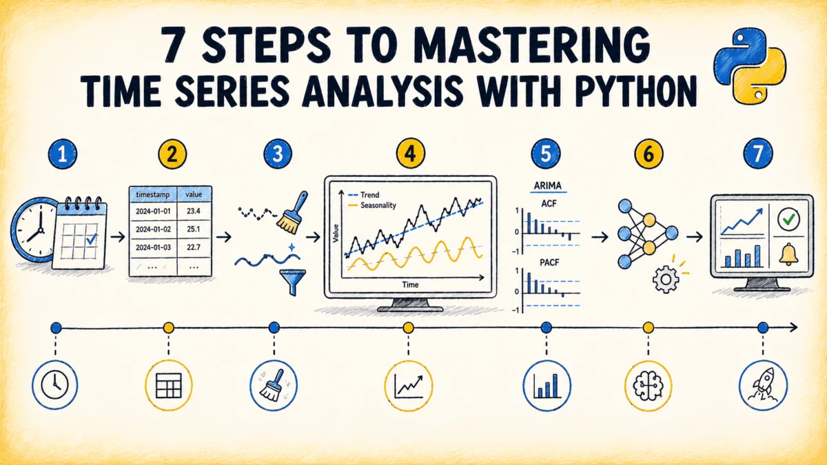
Step 1: Understanding the Foundational Differences of Time Series Data

The initial and arguably most critical step in mastering time series analysis involves a thorough understanding of its unique structural properties. Many practitioners, accustomed to general machine learning paradigms, mistakenly assume a direct transfer of knowledge, often leading to suboptimal or misleading results. Time series data is fundamentally different due to three core properties:

Temporal Dependence: Observations are not independent; the value at any given time point is often correlated with previous values. For example, yesterday’s stock price or last hour’s electricity demand directly influences today’s or the next hour’s values. Standard machine learning models, which typically assume row independence, can produce unreliable forecasts if this dependence is ignored.
Stationarity: A time series is considered stationary if its statistical properties—mean, variance, and autocorrelation structure—remain constant over time. Most classical time series models, such as ARIMA, require stationarity. However, real-world series frequently exhibit non-stationarity, manifesting as trends or changing variability. Addressing non-stationarity, often through differencing or transformations, is a prerequisite for effective modeling.
Seasonality and Trend: These are predictable, systematic components that define the long-run behavior of a series. Trend refers to a long-term increase or decrease in the data, while seasonality describes regular, repeating patterns that occur at fixed intervals (e.g., daily, weekly, monthly, yearly). Separating these systematic components from the irregular, residual noise is often the core analytical challenge, providing crucial insights into the underlying processes generating the data.

Leading experts, such as Rob Hyndman and George Athanasopoulos, in their seminal work "Forecasting: Principles and Practice," emphasize these properties as foundational, recommending a deep dive into them before attempting any modeling. Neglecting these distinct characteristics can lead to models that fail to capture the true dynamics of the data, resulting in poor forecasting performance and unreliable insights.

Step 2: Mastering Time Series Data Structures in Python

Proficiency in time series analysis with Python necessitates a deep comfort with pandas’ time-aware data structures. The library offers robust tools for handling temporal data, including DatetimeIndex, PeriodIndex, and powerful resampling and rolling operations.

DatetimeIndex vs. PeriodIndex: Understanding the distinction between these two index types is crucial. DatetimeIndex represents specific points in time, suitable for irregular or high-frequency data, while PeriodIndex represents fixed-frequency intervals, ideal for regularly spaced data. Knowing when to use each, how to convert between them, and how to parse, slice, and manipulate time-indexed data efficiently prevents significant friction, as many modeling libraries have specific format requirements.
Resampling and Aggregation: This is a common source of subtle yet consequential errors. Downsampling, such as converting minute-level data to hourly data, requires careful selection of aggregation functions (e.g., mean, sum, median, first, last). An incorrect choice can corrupt the analysis by misrepresenting the underlying signal. Practicing various resampling strategies on real datasets until the logic becomes intuitive is an invaluable investment of time.
Rolling and Expanding Windows: Pandas’ .rolling() and .expanding() methods are primitives for generating lag features and cumulative statistics. Building rolling means, standard deviations, and lag offsets manually before relying on higher-level abstractions is critical. This hands-on approach fosters an understanding of what these operations achieve at the index level, preventing a whole class of subtle data leakage errors that are notoriously difficult to diagnose post-factum, especially in forecasting contexts where future information must be strictly excluded.

The official pandas Time Series and Date Functionality guide serves as an indispensable resource for solidifying these fundamental data manipulation skills.

Step 3: Learning to Clean and Prepare Time Series Data

Real-world time series data is rarely pristine, often arriving with missing timestamps, sensor dropouts, duplicate readings, and outliers. Data cleaning in time series is uniquely challenging because temporal ordering constrains every operation, requiring specialized techniques different from those used for tabular data.

Handling Missing Data: A missing timestamp is distinct from a NaN value at an existing timestamp. The former necessitates reindexing to a canonical frequency grid (e.g., hourly, daily) before imputation can accurately locate and fill the gaps. For NaN values, the imputation strategy must align with the gap length and signal type: time-based interpolation (e.g., linear, spline) is suitable for short gaps in continuous signals; forward-fill (or backward-fill) is appropriate for step-function variables like equipment states; and seasonal decomposition imputation can handle longer gaps in strongly seasonal series.
Outlier Detection: Outlier detection in time series requires local rather than global thinking. A value that appears extreme in isolation might be normal within its seasonal context. Techniques like robust decomposition (e.g., STL decomposition) can help identify outliers in the residual component after trend and seasonality are removed. An outlier should be evaluated not just against the series mean but against recent values and typical seasonal patterns.
Frequency Alignment: When merging series recorded at different rates (e.g., hourly meter readings with daily weather data), careful frequency alignment is paramount. The aggregation function chosen during downsampling is as critical as the join operation itself. Documenting the downsampling logic is essential, as the choice profoundly impacts model inputs in ways that are often invisible in the merged output. The sktime library’s transformations documentation offers practical examples for common preprocessing tasks, emphasizing best practices for temporal data.

Step 4: Developing Intuition Through Exploratory Analysis

Before any model can be effectively fit, a thorough exploratory data analysis (EDA) tailored for time series is indispensable. EDA for time series goes beyond simple summary statistics, focusing on revealing the temporal structure of the data.

Decomposition: This should be the first step in any serious analysis. Using functions like statsmodels.tsa.seasonal.seasonal_decompose or the more robust STL decomposition, a time series can be separated into its constituent trend, seasonal, and residual components. Each component then warrants independent examination to understand its behavior and potential anomalies.
Autocorrelation Analysis: The autocorrelation function (ACF) and partial autocorrelation function (PACF) plots are primary tools for understanding temporal dependence.
- ACF shows the correlation of a series with its own lagged values, revealing the overall persistence of patterns.
- PACF measures the correlation between a series and its lagged values after removing the effects of intermediate lags, helping to identify the direct relationship at specific lags.
  Fluently interpreting these plots is essential for identifying autoregressive (AR) and moving average (MA) components, which are foundational for classical modeling.
Stationarity Testing: This rounds out the exploratory workflow. The Augmented Dickey-Fuller (ADF) test and the Kwiatkowski–Phillips–Schmidt–Shin (KPSS) test provide statistical evidence for or against stationarity. Running both tests is advisable as they evaluate complementary hypotheses. The results directly inform whether differencing or other transformations are necessary before modeling can commence, ensuring that subsequent models meet their underlying assumptions. The statsmodels library’s time series analysis documentation provides comprehensive details on these functions.

Step 5: Building Classical Statistical Forecasting Models

Classical statistical models, including ARIMA (Autoregressive Integrated Moving Average), Exponential Smoothing (ETS), and their various extensions, represent the foundational layer of forecasting. They are often surprisingly competitive with more complex approaches on clean, well-understood series and critically, they force a direct engagement with the inherent structure of the data in ways that many machine learning models do not.

Exponential Smoothing (ETS): This is an excellent starting point due to its intuitive nature. ETS models assign exponentially decaying weights to past observations, giving more importance to recent data. They encompass a wide range of behaviors through additive and multiplicative components for trend and seasonality (e.g., Holt-Winters). Fitting an ExponentialSmoothing model from statsmodels.tsa.holtwinters and examining its components provides immediate intuition about the series’ underlying structure.
ARIMA and SARIMA: These models naturally follow. ARIMA models the autocorrelation structure of a stationary series through autoregressive (AR) and moving average (MA) terms, with an ‘Integrated’ (I) component for differencing to achieve stationarity. SARIMA (Seasonal ARIMA) extends this framework to effectively handle seasonal patterns. Identifying the correct orders (p, d, q) for ARIMA and (P, D, Q, S) for SARIMA often relies on the insights gained from ACF and PACF plots and stationarity tests.
Evaluation Discipline: Walk-Forward Validation: Crucially, evaluating time series models demands specific discipline. Random cross-validation, common in general machine learning, produces optimistic and unreliable estimates for time series due to temporal dependence. Walk-forward validation (also known as rolling-origin or time series cross-validation) is the correct approach: train on a segment of historical data, predict the next window, then advance the training window and repeat. This method accurately simulates how the model would perform in a real-world production environment. TimeSeriesSplit from scikit-learn or sktime‘s forecasting cross-validation utilities provide robust implementations of this methodology. "Forecasting: Principles and Practice" chapters on ETS and ARIMA, alongside the statsmodels State Space documentation, offer detailed implementation guidance.

Step 6: Progressing to Machine Learning and Deep Learning Models

Once a solid understanding of classical baselines is established, machine learning (ML) and deep learning (DL) models offer expanded capabilities for handling richer feature sets, complex non-linearities, and scaling to large collections of time series that would be impractical to model individually.

Tree-Based Models (LightGBM, XGBoost): Gradient Boosting Machines like LightGBM and XGBoost are powerful for time series forecasting when provided with well-engineered features. These features typically include lagged values of the target variable, rolling statistics (means, standard deviations, quantiles over various windows), and calendar variables (day of week, month, holiday indicators). These models excel at capturing non-linear relationships and feature interactions automatically. The central risk, however, is data leakage; all lag features must be constructed strictly from past values relative to the prediction timestamp. sktime‘s make_reduction utility wraps scikit-learn regressors as forecasters, safely handling this complex bookkeeping.
Global Models: For problems involving hundreds or thousands of related time series (e.g., store-level sales, device-level sensor data, regional energy demand), training a single global model across all series can significantly outperform individual per-series models by sharing statistical strength and learning common patterns. Frameworks like NeuralForecast are specifically designed to support this pattern natively, facilitating the development of models that generalize well across diverse but related series.
Deep Learning Architectures: Deep learning models, including Recurrent Neural Networks (RNNs) like LSTMs and GRUs, and increasingly Transformer-based architectures, have demonstrated the strongest track records on benchmark datasets. They are particularly adept at handling multi-seasonality, incorporating numerous exogenous covariates, and excelling in long-horizon forecasting tasks. NeuralForecast provides a consistent API for implementing many of these advanced deep learning models with proper temporal cross-validation support. The strategic timing for deploying deep learning is typically after simpler ML models have reached a performance plateau, rather than as an initial approach. The Kaggle M5 Forecasting competition notebooks offer excellent real-world examples of feature engineering and ensembling with advanced ML/DL techniques.

Step 7: Deploying and Monitoring Forecasting Systems

The operational challenges specific to time series forecasting systems are distinct from general machine learning deployment, necessitating specialized attention to ensure reliability and sustained performance.

Concept Drift and Distribution Shift: These are inherent risks, not mere edge cases, in time series, given the non-stationary nature of most real-world data. Economic shifts, technological advancements, or behavioral changes can cause the underlying data generating process to change over time, rendering existing models obsolete. Continuous monitoring of forecast error metrics on a rolling basis, coupled with automated alerts when error rates exceed predefined thresholds, is the absolute baseline. Scheduled retraining pipelines are not optional but fundamental to any production forecasting system, ensuring models adapt to evolving data patterns.
Forecast Storage and Versioning: Production forecasting systems generate predictions continuously. Deliberate design is required for storing these forecasts alongside the actual values they predicted, rather than merely archiving the final model outputs. This comprehensive storage enables the computation of retrospective accuracy at every forecast horizon, providing granular insights into exactly where and why a model’s performance might degrade over time. It also supports robust version control for models and their outputs.
Rigorous Backtesting as a Deployment Gate: Before any forecasting model is deployed live, a rigorous backtest must simulate the full deployment window using only data that would have been available at each prediction step. This means avoiding any look-ahead bias and ensuring that the entire pipeline—from data preprocessing to feature engineering and model inference—is faithfully replicated. A model that performs well on a static held-out test set but fails a proper backtest is not ready for production. Tools like Evidently AI’s model monitoring guide provide frameworks for detecting data and prediction drift, essential for maintaining model health in dynamic environments.

The Future of Time Series Analysis

Mastering time series analysis rewards a sequential, layered learning approach more than most data science disciplines. Each step builds upon the previous, solidifying foundational understanding before progressing to more complex methodologies. From grasping the core properties of temporal dependence and stationarity to navigating Python’s time-aware data structures, diligently cleaning and preparing data, and conducting insightful exploratory analyses, these initial stages form the bedrock. This foundation then enables the effective application of classical statistical models, which provide crucial baselines and structural engagement with the data, before scaling to sophisticated machine learning and deep learning models capable of handling rich feature sets and large collections of series. Finally, the operational discipline required for deployment and monitoring—addressing concept drift, ensuring robust storage, and implementing rigorous backtesting—transforms experimental models into reliable production systems.

The emergence of "foundation models" for time series—pre-trained on vast corpora of diverse series and fine-tuned for specific tasks—represents a significant shift in how practitioners approach forecasting. However, building strong fundamentals in classical and machine learning-based approaches remains indispensable. These core skills provide the necessary intuition, diagnostic capabilities, and problem-solving framework to effectively leverage and adapt to new advancements, ensuring robust and interpretable forecasting solutions in an ever-evolving data landscape. The continued evolution of Python libraries and the growing strategic importance of predictive analytics underscore that expertise in time series analysis will remain a highly valued asset for the foreseeable future.