
The Python scientific computing and machine learning ecosystem fundamentally relies on NumPy, a library that serves as the high-performance engine underpinning critical tools such as Pandas, Scikit-Learn, SciPy, and PyTorch. NumPy’s unparalleled speed in numerical operations stems from its core implementation in optimized C and Fortran, allowing it to manipulate contiguous blocks of memory with minimal overhead, bypassing the inherent inefficiencies of Python’s object model and dynamic interpreter. This architectural advantage makes NumPy indispensable for processing large datasets efficiently.
Despite its powerful capabilities, a significant challenge persists: many data scientists and developers inadvertently write NumPy code that fails to fully leverage this inherent power. Common practices, such as translating standard Python loops directly into numerical computations or employing naive calculations that necessitate frequent, unnecessary memory allocations and array copies, invariably introduce performance bottlenecks. When confronted with datasets comprising millions or billions of entries, these inefficiencies are not merely minor inconveniences; they manifest as bloated RAM usage, detrimental cache misses, and drastically extended execution times. To truly unlock the potential for high-performance numerical code, a deep understanding of NumPy’s internal mechanisms—specifically how it manages computation, memory allocation, and data layouts—is paramount. This article delves into three essential NumPy techniques designed to significantly optimize code performance, reduce resource consumption, and enhance scalability in demanding data science applications.
The Performance Imperative: Bridging the Python-C Divide
The divergence in performance between Python’s native execution model and NumPy’s optimized C/Fortran backend is a critical consideration for any data professional. Python, as an interpreted language, introduces overheads with every operation: type checking, method lookups, and dynamic memory management contribute to slower execution speeds, particularly in iterative numerical tasks. NumPy, by contrast, offloads these operations to pre-compiled C routines. When operations are performed on NumPy arrays, the Python interpreter merely initiates the C-level function, which then executes at near-native hardware speeds, often leveraging processor-specific optimizations like Single Instruction, Multiple Data (SIMD) instructions. This architecture allows a single CPU instruction to operate on multiple data points simultaneously, dramatically accelerating computations on large, homogeneous data structures.
The challenge for developers lies in translating a Pythonic mental model, which often involves explicit iteration, into a NumPy-idiomatic approach that capitalizes on these low-level optimizations. Failing to do so negates much of NumPy’s core advantage, leading to code that is functionally correct but severely underperforms, especially when handling the massive datasets characteristic of modern machine learning and big data analytics. The implications extend beyond mere execution time; inefficient memory usage can lead to costly resource over-provisioning in cloud environments, longer development cycles due to slow experimentation, and ultimately, a reduced capacity to scale solutions effectively.
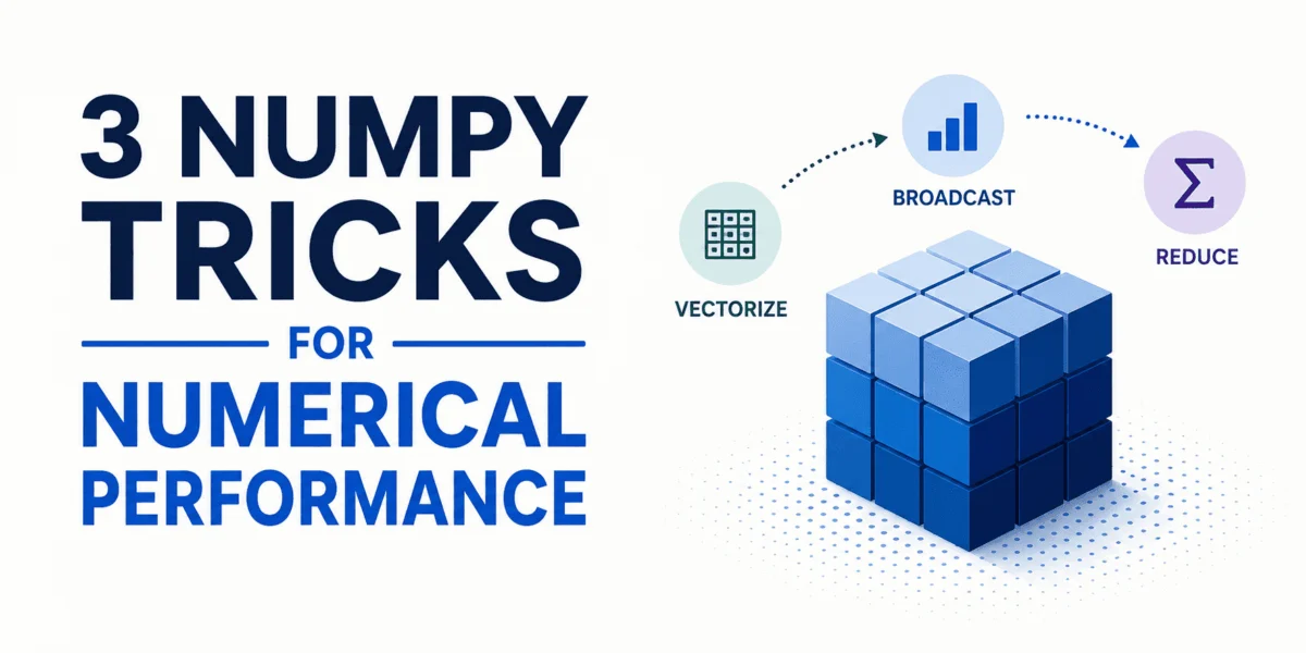
Strategy 1: Harnessing Vectorization and Broadcasting for Speed
One of the most profound performance inhibitors in numerical computing within the Python ecosystem is the explicit Python for loop. Iterating element-by-element through data structures compels the Python interpreter to execute type checking and method lookups at each step, accumulating significant overhead. This "loop tax" is especially punitive when dealing with large arrays.
A common misconception among developers is the utility of np.vectorize. Many assume that wrapping a standard Python function with np.vectorize magically transforms it into optimized C code. This is a critical misunderstanding; np.vectorize is merely a convenience wrapper. It provides a cleaner API for functions that expect scalar inputs but internally still runs a slow, standard Python loop. Consequently, it offers no performance benefits and can even introduce slight overhead due compared to a direct Python loop due to the function call mechanism.
True optimization in this context is achieved by embracing native Universal Functions (ufuncs) and broadcasting. Ufuncs are core NumPy functions (e.g., np.add, np.subtract, np.multiply, np.mean, np.std) that operate element-wise on arrays and are implemented in compiled C. Broadcasting is a powerful mechanism that allows NumPy to perform operations on arrays of different shapes and dimensions without explicitly copying data. Instead, it intelligently "stretches" or "aligns" smaller arrays to match the shape of larger ones, executing the underlying operations directly in compiled C. This conceptual expansion of arrays happens without physical memory duplication, making it incredibly memory-efficient and fast.
Case Study: Column-wise Standardization Benchmark
Consider a scenario requiring column-wise standardization of a large 2D array, a common preprocessing step in machine learning. The goal is to subtract the mean and divide by the standard deviation for each column.
A naive, loop-based approach iterates through the matrix row-by-row and column-by-column:
import numpy as np
import time

# Create a sample matrix (50000 rows, 1000 columns)
matrix = np.random.rand(50000, 1000)

start_time = time.time()

# Naive loop-based column normalization
res = matrix.copy()
for col in range(matrix.shape[1]):
    col_mean = np.mean(matrix[:, col])
    col_std = np.std(matrix[:, col])
    for row in range(matrix.shape[0]):
        res[row, col] = (matrix[row, col] - col_mean) / col_std

duration_loop = time.time() - start_time
print(f"Nested loop processed matrix in: duration_loop:.4f seconds")
Output:
Nested loop processed matrix in: 10.9986 secondsThis execution time, approaching 11 seconds for a matrix of 50 million elements, highlights the significant performance penalty of explicit Python loops. Each iteration incurs the full overhead of Python’s dynamic nature.
In contrast, the vectorized approach leverages NumPy’s ufuncs and broadcasting:
import numpy as np
import time

# Create a sample matrix (50000 rows, 1000 columns)
matrix = np.random.rand(50000, 1000)

start_time = time.time()

# Compute means and standard deviations along axis 0 in compiled C
means = np.mean(matrix, axis=0)
stds = np.std(matrix, axis=0)

# Let broadcasting automatically expand the shapes and compute in one line
res_vectorized = (matrix - means) / stds

duration_vectorized = time.time() - start_time
print(f"Vectorized broadcasting processed matrix in: duration_vectorized:.4f seconds")
Output:
Vectorized broadcasting processed matrix in: 0.1972 secondsThis transformation yields an astounding approximately 56-fold speedup. The vectorized implementation operates on the entire matrix array and the 1D means and stds arrays. NumPy’s broadcasting rules implicitly align the shapes: the (1000,) shaped means array is conceptually expanded across the 50,000 rows of the (50000, 1000) matrix. This expansion occurs instantaneously without data duplication. Crucially, the entire computation—subtraction and division—is pushed down to highly optimized C routines, which exploit SIMD CPU instructions to process multiple data points in parallel. This not only drastically reduces computation time but also improves cache utilization by performing operations on contiguous memory blocks, a fundamental advantage over scattered Python object accesses.
Strategy 2: Mastering In-Place Operations for Memory Efficiency
Beyond raw computational speed, efficient memory management is critical, especially when working with extremely large arrays. Expressions like y = 2 * x + 3 might appear innocuous, but NumPy evaluates such chained operations step-by-step. First, 2 * x is computed, creating a temporary intermediate array to store its result. Then, temp_array + 3 is calculated, creating another temporary array. Finally, this second temporary array is assigned to y.
While manageable for small arrays, this process creates substantial overhead when dealing with arrays containing millions or billions of entries. Each temporary array requires a new memory allocation and subsequent garbage collection. This constant allocation and deallocation pattern "thrashes" the CPU caches, meaning relevant data is frequently evicted from the fast L1/L2 caches, forcing the CPU to fetch data from slower main memory. It also saturates the memory bus bandwidth, becoming a significant bottleneck.
To mitigate this, developers should employ in-place calculations using augmented assignment operators (e.g., *=, +=) or, more robustly, by utilizing the out parameter available in almost all NumPy universal functions. The out parameter allows specifying a pre-allocated array where the result of the operation should be stored, thereby eliminating the need for NumPy to create temporary buffers.
Case Study: Linear Scaling Memory Optimization
Consider a basic linear scaling operation (e.g., y = scale * x + offset) on a massive 1D array.
The naive method, using chained operations, incurs multiple temporary allocations:
import numpy as np
import time

# Create a large 1D array of 10 million elements
x = np.random.rand(10000000)
scale = 2.5
offset = 1.2

start_time = time.time()

# Standard chained math creates temporary intermediate arrays
y_naive = scale * x + offset

duration_naive = time.time() - start_time
print(f"Chained expression executed in: duration_naive:.4f seconds")
Output:
Chained expression executed in: 0.0393 secondsWhile 0.0393 seconds might seem fast, it still involves two full memory allocations for intermediate arrays, each potentially consuming 80MB (10 million floats * 8 bytes/float). For operations performed repeatedly or within memory-constrained environments, this overhead accumulates.
The optimized approach pre-allocates the target output array once and reuses its buffer for all subsequent mathematical operations, completely bypassing temporary allocations:
import numpy as np
import time

# Create a large 1D array of 10 million elements
x = np.random.rand(10000000)
scale = 2.5
offset = 1.2

start_time = time.time()

# Pre-allocate the final array
y_optimized = np.empty_like(x)

# Perform math directly into the target buffer without intermediate variables
np.multiply(x, scale, out=y_optimized)
np.add(y_optimized, offset, out=y_optimized)

duration_optimized = time.time() - start_time

print(f"Optimized in-place expression executed in: duration_optimized:.4f seconds")
print(f"Speedup: duration_naive / duration_optimized:.2fx faster!")
Output:
Optimized in-place expression executed in: 0.0133 seconds
Speedup: 2.95x faster!
In this optimized example, np.multiply(x, scale, out=y_optimized) writes the result of the multiplication directly into the pre-allocated y_optimized array. Subsequently, np.add(y_optimized, offset, out=y_optimized) adds the offset and writes the result back into the same memory buffer. This strategy completely eliminates the need for allocating and garbage-collecting temporary buffers. The benefits are multi-fold: reduced system memory pressure, improved CPU cache locality (as data remains in the same memory region), and a substantial boost in execution speed, nearly tripling performance in this specific benchmark. This practice is particularly vital in memory-intensive applications or when operating within environments with strict memory limits, such as embedded systems or large-scale distributed computing clusters.
Strategy 3: Distinguishing Memory Views from Copies for Resource Management
A nuanced yet critically important aspect of high-performance numerical programming with NumPy involves understanding when an operation returns a view of an array versus a copy. This distinction dictates whether new memory is allocated and data is duplicated, or if a new array object simply references the existing data buffer.
- Views: A view is a new array object that looks at the same data as the original array. No new memory is allocated for the data itself; only a new "header" or metadata structure is created. Changes made to the view will directly affect the original array, and vice-versa.
- Copies: A copy is a completely independent new array object with its own distinct data buffer. Changes to a copy do not affect the original array.
The rule of thumb is that basic slicing (using start, stop, and step indices, e.g., arr[0:10:2] or arr[::2]) always returns a view. This is incredibly efficient as it avoids data duplication. In contrast, advanced indexing (using lists of indices or boolean masks, e.g., arr[[0, 2, 4]] or arr[arr > 0.5]) always returns a copy. This is because advanced indexing often involves non-contiguous memory access patterns, making it impossible to represent the result as a simple view of the original contiguous block.
Unnecessary memory copies, particularly when working with large arrays, can trigger massive and avoidable memory allocations, consuming significant RAM and introducing performance penalties due to data transfer.
Case Study: Sub-sampling a Matrix Benchmark
Consider the task of sub-sampling a large 2D matrix, extracting every second row and column.
Using advanced indexing, by passing lists of integer indices, forces NumPy to allocate a large new array and physically copy all the elements:
import numpy as np
import time

# Create a matrix of 10,000 x 10,000 elements (100 million elements)
matrix = np.random.rand(10000, 10000)

start_time = time.time()

# Advanced indexing using integer arrays forces a physical copy of data
rows = np.arange(0, matrix.shape[0], 2)
cols = np.arange(0, matrix.shape[1], 2)
sub_matrix_copy = matrix[rows[:, None], cols] # Using None to enable broadcasting for row/column selection

duration_copy = time.time() - start_time
print(f"Advanced indexing copy completed in: duration_copy:.4f seconds")
Output:
Advanced indexing copy completed in: 0.1575 secondsThis operation, taking approximately 0.16 seconds, involves allocating new memory for a 5,000 x 5,000 matrix (25 million elements), which translates to 200MB of new memory (25M * 8 bytes/float). This allocation and data transfer contribute directly to the measured duration.
Now, performing the same sub-sampling using basic slicing:
import numpy as np
import time

# Create a matrix of 10,000 x 10,000 elements
matrix = np.random.rand(10000, 10000)

start_time = time.time()

# Basic slicing returns a zero-copy view instantly
sub_matrix_view = matrix[::2, ::2]

duration_view = time.time() - start_time
print(f"Basic slicing view completed in: duration_view:.8f seconds")
Output:
Basic slicing view completed in: 0.00001001 secondsThe difference is stark: the basic slicing operation completes in approximately 10 microseconds, a staggering 15,000 times faster than the advanced indexing approach. When matrix[::2, ::2] is executed, NumPy does not interact with the underlying data buffer at all. Instead, it creates a new array header (a Python object) that contains modified metadata: a new shape (5000, 5000) and new strides. Strides define the number of bytes to step in each dimension to find the next element. For matrix[::2, ::2], the strides are adjusted to effectively "skip" elements, pointing to the original data at every second row and column. This metadata manipulation is an incredibly lightweight operation, taking only microseconds, regardless of the matrix’s size.
The trade-off for this immense speed and memory efficiency is that the view shares the same memory buffer as the original array. Consequently, any modifications made to sub_matrix_view will directly alter the original matrix. Developers must be acutely aware of this shared memory behavior. If an independent copy is required to prevent unintended side effects on the original data, an explicit call to .copy() must be made (e.g., sub_matrix_copy_safe = matrix[::2, ::2].copy()). Understanding this distinction is crucial for both performance and data integrity in large-scale numerical computations.
Broader Implications and Industry Best Practices
The integration of these three performance design patterns—vectorization and broadcasting, in-place operations, and mindful handling of views vs. copies—transcends mere code optimization; it profoundly impacts the scalability, cost-efficiency, and overall viability of data processing pipelines in real-world production environments.
Scalability for Big Data: As datasets grow from gigabytes to terabytes and beyond, the difference between an optimized NumPy routine and a naive one can be the difference between a task completing in minutes versus hours, or even days. Efficient memory use prevents out-of-memory errors and allows larger datasets to be processed within existing hardware constraints. This is particularly relevant in domains like genomics, high-frequency trading, and large-scale simulations, where data volumes are immense.
Cost Savings in Cloud Computing Environments: Cloud resources are billed based on usage—CPU time, memory consumption, and network bandwidth. Inefficient NumPy code translates directly into longer run times and higher memory footprints, leading to significantly increased operational costs for cloud-hosted data processing jobs. By optimizing code, organizations can reduce their cloud expenditure, making their data science initiatives more economically sustainable.
Impact on Development Cycles and Project Timelines: Faster code execution accelerates the iterative development process. Data scientists can experiment with more models, parameters, and preprocessing steps in less time, leading to quicker insights and faster time-to-market for AI/ML solutions. The ability to prototype and test complex algorithms efficiently is a competitive advantage.
The Role of Developer Education: The pervasive nature of Python in data science means many practitioners come from backgrounds without deep exposure to low-level memory management or CPU architecture. The principles discussed here are not always intuitive when transitioning from standard Python. Industry leaders and educational institutions consistently emphasize the importance of training data professionals in these advanced NumPy concepts to ensure the development of robust, high-performance systems. The NumPy development team’s design philosophy, prioritizing speed and memory efficiency, underscores the library’s role as a critical tool that demands a deeper understanding for optimal utilization.
NumPy’s role as the backbone for the broader scientific Python ecosystem means that improvements in its usage propagate across dependent libraries. When a Pandas operation leverages an optimized NumPy array underneath, or a Scikit-learn algorithm executes faster due to better memory access, the entire ecosystem benefits. This foundational library enables the rapid advancements seen in machine learning, scientific research, and data analytics today.
Wrapping Up
Writing clean, performant NumPy code demands a shift in mindset—moving away from traditional Pythonic iteration and memory handling towards embracing native NumPy mechanics. By consciously avoiding standard Python concepts where NumPy alternatives exist, developers can systematically eliminate computational bottlenecks.
To recap the core strategies:
- Prioritize Vectorization and Broadcasting: Always prefer NumPy’s universal functions and broadcasting over explicit Python
forloops. This pushes computation to optimized C code, leveraging SIMD instructions and vastly improving execution speed. - Embrace In-Place Operations: Minimize temporary array allocations by utilizing in-place operators (
*=,+=) or theoutparameter in NumPy ufuncs. This conserves memory, enhances CPU cache utilization, and boosts performance by reducing memory bus saturation and garbage collection overhead. - Understand Memory Views vs. Copies: Differentiate between basic slicing (which creates zero-copy views) and advanced indexing (which creates full data copies). Opt for views when only reading or modifying sub-segments without needing an independent copy, and explicitly call
.copy()when data independence is paramount.
Integrating these three performance design patterns is crucial for crafting data processing pipelines that are lean, fast, and scalable for demanding production workloads, ensuring that the full power of NumPy is harnessed for modern data science challenges.
Matthew Mayo (@mattmayo13) holds a master’s degree in computer science and a graduate diploma in data mining. As managing editor of KDnuggets & Statology, and contributing editor at Machine Learning Mastery, Matthew aims to make complex data science concepts accessible. His professional interests include natural language processing, language models, machine learning algorithms, and exploring emerging AI. He is driven by a mission to democratize knowledge in the data science community. Matthew has been coding since he was 6 years old.