The intricate world of machine learning, while promising revolutionary advancements, often presents a steep learning curve for newcomers. A fundamental concept frequently oversimplified or explained retrospectively in introductory materials is the "loss function." Far from being a mere mathematical formality, loss functions are the indispensable compasses guiding machine learning models, providing the critical feedback mechanism that enables them to learn from their mistakes and incrementally improve performance. Understanding their role is paramount to comprehending the entire training paradigm of artificial intelligence.
The Foundational Role of Loss Functions
At its core, a machine learning model is an algorithm designed to identify patterns in data and make predictions or decisions. Whether it’s forecasting stock prices, identifying objects in images, or determining the sentiment of text, the model’s initial attempts are often riddled with inaccuracies. The question then arises: how does a model quantify its errors, and how does it know in which direction to adjust its internal parameters to minimize those errors? This is precisely where loss functions come into play.
In essence, a loss function computes a single numerical value that quantifies the "badness" or "discrepancy" between the model’s predicted output and the true, actual value for a given data point. This numerical score, often referred to as the "error" or "cost" for a single instance, serves as the immediate feedback signal. A higher loss value indicates a greater deviation from the correct answer, signaling a significant mistake. Conversely, a lower loss value signifies that the model’s prediction is closer to the ground truth, indicating a more accurate or well-calibrated output.
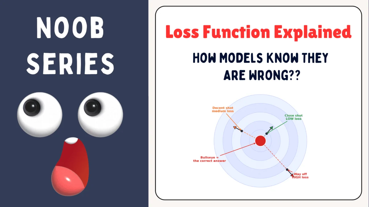
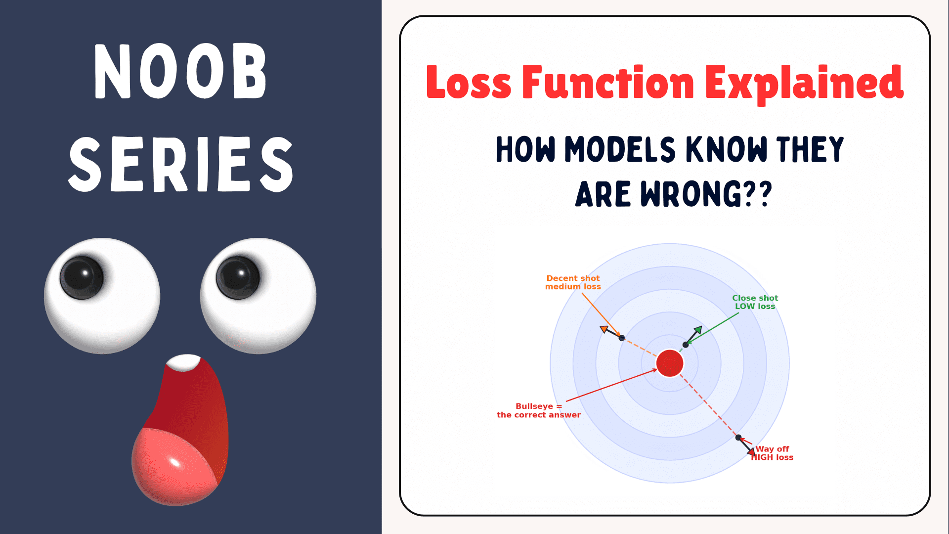
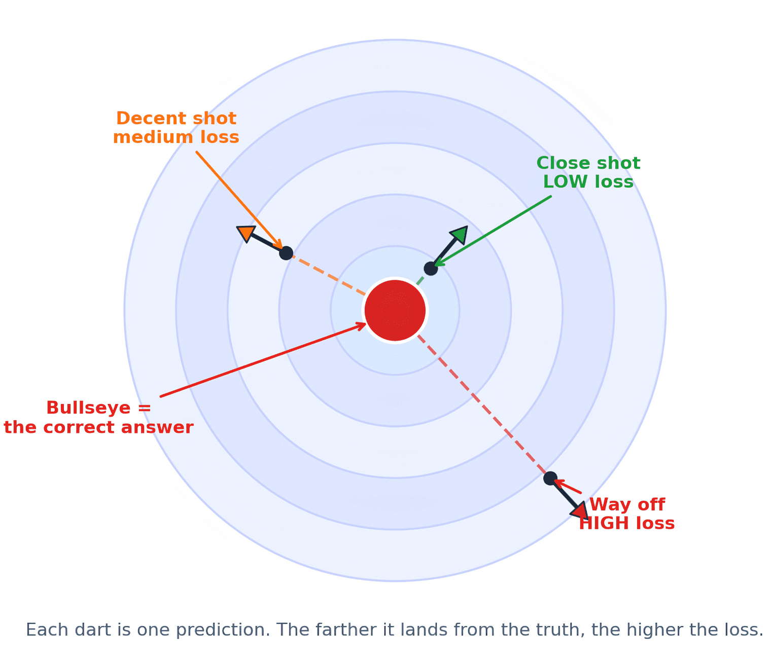
This concept is analogous to a dart player aiming for a bullseye. Each throw is a prediction. Without knowing how far off the dart landed—too high, too low, too far left, or too far right—the player cannot adjust their aim for the next throw. The distance from the bullseye provides the essential feedback required for improvement. In machine learning, the "bullseye" is the correct answer, the "dart" is the model’s prediction, and the "distance" is precisely what the loss function measures. This iterative process of making a prediction, measuring the loss, and adjusting based on that feedback forms the bedrock of how machine learning models learn.
Defining the "Mistake Score": Loss, Cost, and Objective Functions
While often used interchangeably in casual discourse, it is important to clarify the subtle distinctions between "loss function," "cost function," and "objective function" in a professional context.
- Loss Function: Typically refers to the error calculation for a single training example. It quantifies how poorly the model performs on that specific instance.
- Cost Function: More broadly, a cost function (or empirical risk) is the average of the loss functions over the entire training dataset or a batch of training examples. It’s the aggregate measure of the model’s performance across multiple instances. During training, the goal is often to minimize this cost function.
- Objective Function: This is the most general term, encompassing the function that a model seeks to optimize (either minimize or maximize) during training. It can include the cost function, but also additional terms like regularization components (e.g., L1 or L2 regularization) that penalize model complexity to prevent overfitting. Therefore, while minimizing the cost function is a common objective, the objective function provides a more comprehensive view of what the model is truly trying to achieve.
The machine learning community widely acknowledges that a clear understanding of these distinctions, particularly the role of the loss function, is crucial for both theoretical comprehension and practical application. Experts underscore the importance of selecting an appropriate loss function, as it directly dictates the learning process and the ultimate behavior of the trained model.
The Iterative Learning Cycle: Loss Functions in Training
The training of a machine learning model is an iterative dance between prediction, error measurement, and parameter adjustment. This cycle, often referred to as the "training loop," heavily relies on the loss function.
- Forward Pass (Prediction): The model takes an input and generates a prediction.
- Loss Calculation: The predicted output is compared to the actual target value using a chosen loss function. This yields a single numerical value representing the error.
- Backward Pass (Gradient Computation): This is where calculus comes into play. The loss value is used to calculate the "gradients" of the loss function with respect to each of the model’s internal parameters (weights and biases). A gradient indicates the direction and magnitude of the steepest ascent of the loss function. To minimize loss, the model needs to move in the opposite direction.
- Parameter Update (Optimization): An optimization algorithm (e.g., Stochastic Gradient Descent, Adam, RMSprop) utilizes these gradients to adjust the model’s parameters. The parameters are updated in a direction that is expected to reduce the loss in the next iteration. The "learning rate" hyperparameter controls the size of these adjustment steps.
This cycle repeats thousands, even millions, of times over the training data. Initially, with randomly initialized parameters, the model makes numerous errors, resulting in a high loss. As training progresses, the model continuously refines its parameters, leading to a gradual decrease in the loss value. A healthy training curve typically shows a sharp initial drop in loss, followed by a more gradual flattening as the model converges towards an optimal set of parameters. This flattening signifies that the model has learned the predominant patterns and is making finer adjustments. However, if training loss continues to decrease while validation loss (loss on unseen data) begins to rise, it signals overfitting—a critical issue where the model memorizes the training data rather than generalizing patterns.
Key Regression Loss Functions: Quantifying Numerical Deviations
Regression tasks involve predicting continuous numerical values, such as house prices, temperature forecasts, or delivery times. For these problems, the choice of loss function directly impacts how errors are penalized.
Mean Squared Error (MSE): Penalizing Magnitude
One of the most widely used loss functions for regression is the Mean Squared Error (MSE), also known as L2 Loss. Its mathematical formulation is straightforward: it calculates the average of the squares of the differences between predicted and actual values.
The Python representation would be:
def mean_squared_error(predictions, actuals):
    squared_errors = [(p - a) ** 2 for p, a in zip(predictions, actuals)]
    return sum(squared_errors) / len(squared_errors)
The decision to square the errors is driven by two primary considerations:
- Magnitude Sensitivity: Squaring penalizes larger errors much more significantly than smaller errors. For instance, an error of 10 contributes 100 to the total loss, whereas an error of 1 contributes only 1. This characteristic makes MSE suitable when large errors are particularly undesirable and should be heavily penalized.
- Differentiability: The squaring operation results in a smooth, convex function that is continuously differentiable. This property is crucial for optimization algorithms like gradient descent, which rely on calculating gradients to find the minimum loss efficiently. Without differentiability, computing gradients would be challenging, hindering the learning process.
However, MSE’s sensitivity to large errors also makes it susceptible to outliers. A few extreme data points can disproportionately inflate the MSE, leading the model to adjust its parameters excessively to accommodate these outliers, potentially at the expense of overall performance on the majority of the data.
Mean Absolute Error (MAE): Robustness to Outliers
Another common loss function for regression is the Mean Absolute Error (MAE), or L1 Loss. Unlike MSE, MAE calculates the average of the absolute differences between predictions and actual values.
The Python representation is:
def mean_absolute_error(predictions, actuals):
    absolute_errors = [abs(p - a) for p, a in zip(predictions, actuals)]
    return sum(absolute_errors) / len(absolute_errors)
MAE offers a distinct advantage: it treats all errors linearly. An error of 10 contributes 10 to the total loss, and an error of 1 contributes 1. This linear penalty makes MAE more robust to outliers compared to MSE. If a dataset contains a few anomalous data points, MAE will not be as heavily influenced by them, allowing the model to focus on the overall trend of the majority data. This makes MAE a preferred choice in scenarios where outliers are common and should not dictate the model’s learning, such as financial forecasting with occasional extreme market fluctuations.
However, MAE has its own drawbacks. The absolute value function is not differentiable at zero. While most optimization libraries handle this gracefully, it can theoretically pose challenges for gradient-based optimization algorithms when the error is exactly zero. Furthermore, since MAE treats all errors equally, it might not sufficiently penalize very large errors if the application demands strict accuracy for all predictions, regardless of magnitude.
The Hybrid Approach: Huber Loss
To mitigate the respective weaknesses of MSE and MAE, the Huber Loss function (also known as Smooth L1 Loss) was introduced. Huber Loss is a hybrid that behaves like MSE for small errors and like MAE for large errors. It achieves this by defining a threshold, often denoted as delta ($delta$).
- For errors smaller than $delta$, Huber Loss squares the error, similar to MSE.
- For errors larger than $delta$, it takes the absolute value, similar to MAE, but with a linear scaling factor to maintain differentiability at the transition point.
This piecewise function offers a balance: it leverages the differentiability and stronger penalty of MSE for common, small errors, while gaining the robustness to outliers of MAE for infrequent, large errors. Huber Loss is particularly useful in applications where a balance between sensitivity to overall accuracy and robustness to extreme values is desired.
Navigating Categorical Predictions: Cross-Entropy Loss
When models predict categories instead of continuous numbers—such as classifying emails as spam or not, identifying animals in images, or detecting fraudulent transactions—regression loss functions are unsuitable. For these "classification" tasks, models typically output probabilities for each possible category. For example:
Dog: 70%
Cat: 20%
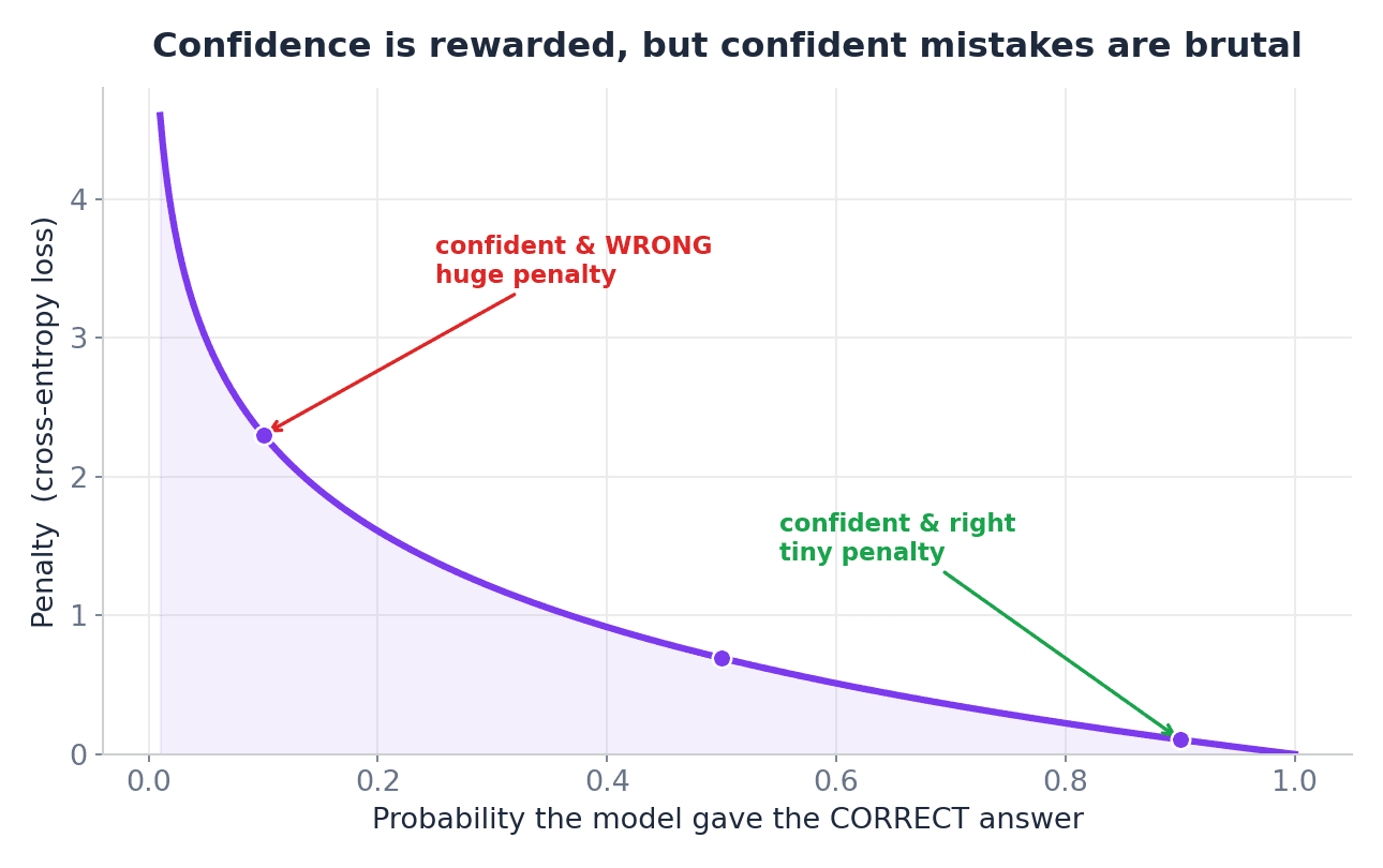
Fish: 10%In such scenarios, the model needs to be penalized not just for being wrong, but for how confident it was in a wrong prediction, or how unconfident it was in a correct prediction. This is where Cross-Entropy Loss (also known as Log Loss) becomes the standard.

Cross-Entropy Loss originates from information theory and measures the difference between two probability distributions: the true distribution (where the correct class has a probability of 1 and others 0) and the predicted distribution (the probabilities output by the model). The core intuition is:
- Penalize confident wrong predictions heavily: If the model predicts a 90% chance of an image being a dog, but it’s actually a cat, the loss will be very high.
- Reward confident correct predictions: If the model predicts an 80% chance of an image being a dog, and it truly is a dog, the loss will be very low.
- Modestly penalize unconfident correct predictions: If the model predicts a 40% chance of an image being a dog, and it’s a dog, the loss will be moderate.
Cross-Entropy Loss is calculated using logarithms, which amplify penalties for probabilities close to zero for the correct class and keep penalties low for probabilities close to one for the correct class.
Binary Cross-Entropy (BCE): Used for binary classification problems (two classes, e.g., spam/not spam). The model outputs a single probability (e.g., probability of being spam), and BCE measures the divergence between this predicted probability and the true binary label (0 or 1).
Categorical Cross-Entropy (CCE): Used for multi-class classification problems (more than two classes, e.g., cat/dog/fish). The model outputs a probability distribution over all classes, and CCE compares this to the one-hot encoded true label (e.g., [0, 1, 0] for cat).
The prevalence of Cross-Entropy Loss in classification tasks underscores its efficacy in fostering models that are not only accurate but also well-calibrated in their probabilistic outputs. It ensures that models learn to assign high confidence to correct predictions and low confidence to incorrect ones, a crucial aspect for reliable AI systems.
Beyond Simple Correctness: Loss vs. Accuracy and Other Metrics
A common point of confusion for beginners is the distinction between "loss" and "accuracy." While both relate to model performance, they measure different aspects and serve different purposes.
- Accuracy: This is a straightforward metric that tells you the proportion of predictions that were precisely correct. For classification, it’s the number of correct classifications divided by the total number of predictions. For regression, it might refer to predictions within a certain tolerance.
- Loss: As established, loss quantifies the magnitude or severity of the model’s mistakes. It provides a continuous, differentiable signal that is essential for guiding the optimization process.
Consider two classification models, Model A and Model B, both achieving 90% accuracy on a dataset. On the surface, they appear equally proficient. However, their loss values could tell a different story. Model A might have been very confident (e.g., 99% probability) on its correct predictions and only slightly wrong (e.g., 55% probability) on its incorrect ones. Model B, conversely, might have been barely correct (e.g., 51% probability) on many examples and extremely confident (e.g., 95% probability) when it was wrong. In this scenario, Model A would likely exhibit a significantly lower Cross-Entropy Loss than Model B, indicating better calibration and more reliable predictions, despite identical accuracy.
This example highlights why loss is the primary metric for training, while accuracy (along with other metrics like precision, recall, F1-score for classification, or R-squared for regression) is typically used for evaluation and human interpretability. Loss functions provide the necessary gradient signal for learning, whereas evaluation metrics offer a more intuitive summary of the model’s practical utility.
Optimizing for Performance: The Role of Gradients and Regularization
The journey of minimizing the loss function is intricately linked to the field of optimization. Once the loss function calculates the error, the next step is to figure out how to adjust the model’s parameters to reduce that error. This is achieved through gradient-based optimization algorithms. These algorithms compute the gradient of the loss function with respect to each model parameter. The gradient points in the direction of the steepest increase in loss. To minimize loss, the model’s parameters are updated in the opposite direction of the gradient.
Furthermore, the objective function often includes not just the loss term but also regularization terms. Regularization techniques like L1 (Lasso) and L2 (Ridge) are added to the loss function to penalize model complexity. This encourages the model to learn simpler patterns and prevents it from overfitting to the training data. For example, in L2 regularization, a term proportional to the square of the magnitude of the model’s weights is added to the loss function. This encourages smaller weights, effectively smoothing the model and improving its generalization capability to unseen data. This combined objective function ensures that the model not only performs well on the training data but also maintains its predictive power on new, unobserved data.
Strategic Selection and Future Outlook: Challenges and Best Practices
The choice of a loss function is not a trivial decision; it is a strategic one that profoundly impacts a model’s learning behavior, its robustness, and its suitability for a specific application. Data scientists and machine learning engineers must carefully consider:
- Problem Type: Regression, classification (binary or multi-class), ranking, generative tasks each have their optimal loss functions.
- Data Characteristics: The presence of outliers, imbalanced classes, or specific error distributions can steer the choice towards MAE over MSE, or necessitate weighted loss functions.
- Desired Model Behavior: Is it critical to heavily penalize large errors (MSE), or is robustness to outliers more important (MAE, Huber)? Should the model be well-calibrated in its probabilities (Cross-Entropy)?
- Computational Efficiency: While less of a concern with modern hardware, the computational cost and differentiability properties of a loss function are practical considerations.
The continuous evolution of machine learning also sees the development of new and specialized loss functions. For instance, in generative adversarial networks (GANs), the loss functions are designed to create a competitive dynamic between a generator and a discriminator. In object detection, specialized losses like Focal Loss address issues of class imbalance. These innovations highlight that while fundamental loss functions remain critical, the field is constantly adapting to new challenges and complex model architectures.
Conclusion: The Indispensable Compass of Machine Learning
In conclusion, the loss function is far more than a mathematical formula; it is the fundamental mechanism through which machine learning models learn. It provides the crucial feedback signal, quantifying the model’s errors and guiding its iterative adjustments. From the magnitude-sensitive Mean Squared Error for regression to the confidence-aware Cross-Entropy for classification, each loss function is meticulously designed to optimize model performance for specific tasks.
Understanding loss functions unlocks a deeper comprehension of various advanced machine learning concepts, including gradient descent, backpropagation, optimization algorithms, and the nuances of preventing overfitting. It transforms the seemingly abstract process of "training a model" into a clear, goal-oriented endeavor: to continuously minimize this mistake score. As artificial intelligence continues to permeate various sectors, a solid grasp of these foundational elements becomes increasingly vital for developing robust, reliable, and ethically sound AI systems. The loss function, truly, is the indispensable compass that navigates the complex landscape of machine learning, guiding models toward ever-greater precision and utility.